Optimized Deployment of Mistral7B on Amazon SageMaker Real-Time Inference

Utilize large model inference containers powered by DJL Serving & Nvidia TensorRT

The Generative AI space continues to expand at an unprecedented rate, with the introduction of more Large Language Model (LLM) families by the day. Within each family there are also varying sizes of each model, for instances there’s Llama7b, Llama13B, and Llama70B. Regardless of the model that you select, the same challenges arise for hosting these LLMs for inference.

The size of these LLMs continue to be the most pressing challenge, as it’s very difficult/impossible to fit many of these LLMs onto a single GPU. There are a few different approaches to tackling this problem, such as model partitioning. With model partitioning you can use techniques such as Pipeline or Tensor Parallelism to essentially shard the model across multiple GPUs. Outside of model partitioning, other popular approaches include Quantization of model weights to a lower precision to reduce the model size itself at a cost of accuracy.

While the model size is a large challenge in itself, there is also the challenge of retaining the previous inference/attention in Text Generation for Decoder based models. Text Generation with these models is not as simple as traditional ML model inference where there is just an input and output. To calculate the next word in text generation, the state/attention of the previously generated tokens must be retained to provide a logical output. The storing of these values is known as the KV Cache. The KV Cache enables you to cache the previously generated tensors in GPU memory to generate the next tokens. The KV Cache also takes up a large amount of memory that needs to be accounted for during model inference.

To address these challenges many different model serving technologies have been introduced such as vLLM, DeepSpeed, FasterTransformers, and more. In this article we specifically look at Nvidia TensorRT-LLM and how we can integrate the serving stack with DJL Serving on Amazon SageMaker Real-Time Inference to efficiently host the popular Mistral 7B Model.

NOTE: This article assumes an intermediate understanding of Python, LLMs, and Amazon SageMaker Inference. I would suggest following this article for getting started with Amazon SageMaker Inference. To understand more about LLM Hosting/Inference specifically I would refer here.

DISCLAIMER: I am a Machine Learning Architect at AWS and my opinions are my own.

Model Serving Stack
Mistral Deployment
Load Testing & AutoScaling
Additional Resources & Conclusion

1. Model Serving Stack

SageMaker Inference integrates natively with a variety of different Model Servers via the managed containers that are provided via ECR. For this example, we will specifically use the Large Model Inference (LMI) containers that are powered by DJL Serving.

DJL Serving is a high performant model serving solution that provides various features that help optimize LLM deployments specifically. With the DJL model server you can specify a runtime engine that will allow for you to work with different model partitioning frameworks such as Accelerate, DeepSpeed, and in this case specifically TensorRT LLM.

For the purpose of this example we will retrieve the latest LMI container (0.26.0 at the time of this writing), and specify the TensorRT framework. This enables us to work with the optimizations enabled via this framework such as Tensor Parallel, Server Side Batching, and more that we will explore in the example.

While we use DJL Serving via the LMI containers in this example, you can choose the model server/container that is most appropriate for your use-case. If you do choose to use LMI, understand the frameworks that are available to choose what is best suited for your use-case.

2. Mistral Deployment

For this example we will be working in a ml.c5.xlarge SageMaker Classic Notebook Instance with a conda_python3 kernel. We first setup credentials with the SageMaker Python SDK which we will be using for endpoint creation and orchestration:

import boto3
import sagemaker
from sagemaker import Model, image_uris, serializers, deserializers

role = sagemaker.get_execution_role()  # execution role for the endpoint
sess = sagemaker.session.Session()  # sagemaker session for interacting with different AWS APIs
region = sess._region_name  # region name of the current SageMaker Studio environment
account_id = sess.account_id()

To specify our serving optimizations, DJL expects a serving.properties file with the tuned configuration. In this case we specify a few different parameters:

Tensor Parallel: As we discussed most of these LLMs cannot fit into a single GPU machine. With Tensor Parallel the model is sharded across layers (intra-layer). You can define this value as the number of GPUs that are available for the instance type for deployment. In this case we use an ml.g5.12xlarge which has four GPUs so we specify that value.
Rolling/Continuous Batching: Server Side Batching is a popular technique utilized to improve the throughput of applications. Rather than taking an individual request at a time, a batch of requests is processed, you can also define the max batch size within the properties file. Traditionally, the server waits for this batch to be completed, before proceeding to take on the next batch. With LLMs this can lead to lower GPU Utilization and longer wait times as the entire batch needs to be processed. Continuous/Rolling Batching is a technique in which we do not wait for the batch to be completed rather we actively pushes new requests into a batch and release finished sequences. To understand further about Batching techniques, please refer to the Llama Batching blog here, a key concept in Paged Attention Batching is covered as well.

We now define the serving.properties file for deploying Mistral7B. Note that we specify the HuggingFace Model ID, the model server will directly pull down the model data and artifacts into S3 rather than your local machine where you are working. In the case that you have your own model artifacts, you can specify the S3 path in the model_id variable location.

%%writefile serving.properties
engine=MPI
option.tensor_parallel_degree=4
option.model_id=mistralai/Mistral-7B-v0.1
option.max_rolling_batch_size=16
option.rolling_batch=auto

The process for creating a SageMaker Endpoint is now very similar to deploying a traditional ML model on SageMaker. We create a tarball with the serving properties file and specify the TensorRT LLM container.

%%sh
# create model.tar.gz for deployment
mkdir mymodel
mv serving.properties mymodel/
tar czvf mymodel.tar.gz mymodel/
rm -rf mymodel

# retreive TensorRT image
image_uri = image_uris.retrieve(
        framework="djl-tensorrtllm",
        region=sess.boto_session.region_name,
        version="0.26.0"
    )

# upload model data to S3
s3_code_prefix = "large-model-lmi/code"
bucket = sess.default_bucket()  # bucket to house artifacts
code_artifact = sess.upload_data("mymodel.tar.gz", bucket, s3_code_prefix)
print(f"S3 Code or Model tar ball uploaded to --- > {code_artifact}")

We then deploy our SageMaker Model object with the S3 path to the serving file and the container image we have specified. In this case we use a ml.g5.12xlarge instance with four available GPUs:

model = Model(image_uri=image_uri, model_data=code_artifact, role=role)

# this step can take around ~ 10 minutes for creation, the model artifacts are being pulled from HF Hub
instance_type = "ml.g5.12xlarge"
endpoint_name = sagemaker.utils.name_from_base("lmi-trt-mistral")

model.deploy(initial_instance_count=1,
             instance_type=instance_type,
             endpoint_name=endpoint_name
            )

# our requests and responses will be in json format so we specify the serializer and the deserializer
predictor = sagemaker.Predictor(
    endpoint_name=endpoint_name,
    sagemaker_session=sess,
    serializer=serializers.JSONSerializer(),
)

Endpoint creation will take around ten minutes, as the model artifacts will be pulled from the HuggingFace Hub Model ID we specified. Once created, we can then run a sample inference either using the SageMaker Python SDK or the lower level Boto3 Python SDK.

# inference via sagemaker python SDK
predictor.predict(
    {"inputs": "Who is Roger Federer?"})

# boto3 inference sample
import json
runtime_client = boto3.client('sagemaker-runtime')
content_type = "application/json"
payload = {"inputs": "Who is Roger Federer?"} #optionally add any parameters for your model

# sample inference
response = runtime_client.invoke_endpoint(
    EndpointName=endpoint_name,
    ContentType=content_type,
    Body=json.dumps(payload))
result = json.loads(response['Body'].read().decode())['generated_text']
print(result)

Now that our endpoint is responsive, let’s see how we can load test our model.

3. Load Testing & AutoScaling

For Load Testing, we will use a familiar tool known as Locust. Locust is an open-source Python load testing tool that will allow you to define a point of contact, also known as a Task. The Locust Task that we will be measuring is the invoke_endpoint API call we earlier defined. To further understand using Locust to load-test SageMaker Endpoints please refer to this blog.

For LLMs we want to consider a few points before load testing. What are the different payload sizes we should expect for our model? What is the maximum context window of our model? These questions are important as uneven payload sizes can lead to different response times and model behavior.

To simulate a realistic use-case we’ve defined an array of sample questions/prompts in our Locust file that sets up our load test. At the point of invocation, a random question will be chosen from the array. For your model and your load tests, replace the prompts in this array with what you would expect for your production traffic.

class BotoClient:
    def __init__(self, host):
        # Consider removing retry logic to get accurate picture of failure in locust
        config = Config(
            region_name=region, retries={"max_attempts": 0, "mode": "standard"}
        )

        self.sagemaker_client = boto3.client("sagemaker-runtime", config=config)
        self.endpoint_name = host.split("/")[-1]
        self.content_type = content_type
        # replace with your inputs
        self.sampPayloads = [
            "Who is Roger Federer?",
            "What is the capitol of the United States?",
            "What is the capitol of India?",
            "Who is LeBron James?",
            "Where was pizza first made?"]
        # random prompt is chosen
        self.payload = json.dumps({"inputs": random.choice(self.sampPayloads)})

We then parameterize this load test with a shell script where you can increase the users and workers to generate further traffic. Note that you will be constrained to the number of workers that are available on the machine that you are conducting the load test on.

#replace with your endpoint name in format https://<<endpoint-name>>
export ENDPOINT_NAME=https://$1

export REGION=us-east-1
export CONTENT_TYPE=application/json
export USERS=20
export WORKERS=5
export RUN_TIME=1mg # adjust to change duration of test
export LOCUST_UI=false # Use Locust UI

We can then execute this shell script in our notebook to see the load test kicked off.

%%bash -s "$endpoint_name"
./distributed.sh $1

Post the test (we set one minute as a default), you will see metrics generated in a CSV file to summarize the test.

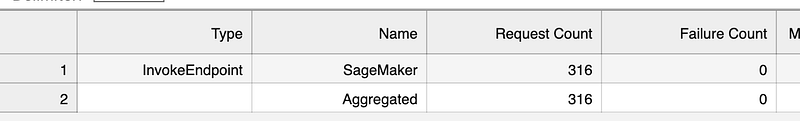
We can also validate these metrics via the built-in CloudWatch diagrams in the SageMaker Endpoint UI. Here we can also get a better understanding of how saturated our hardware is.

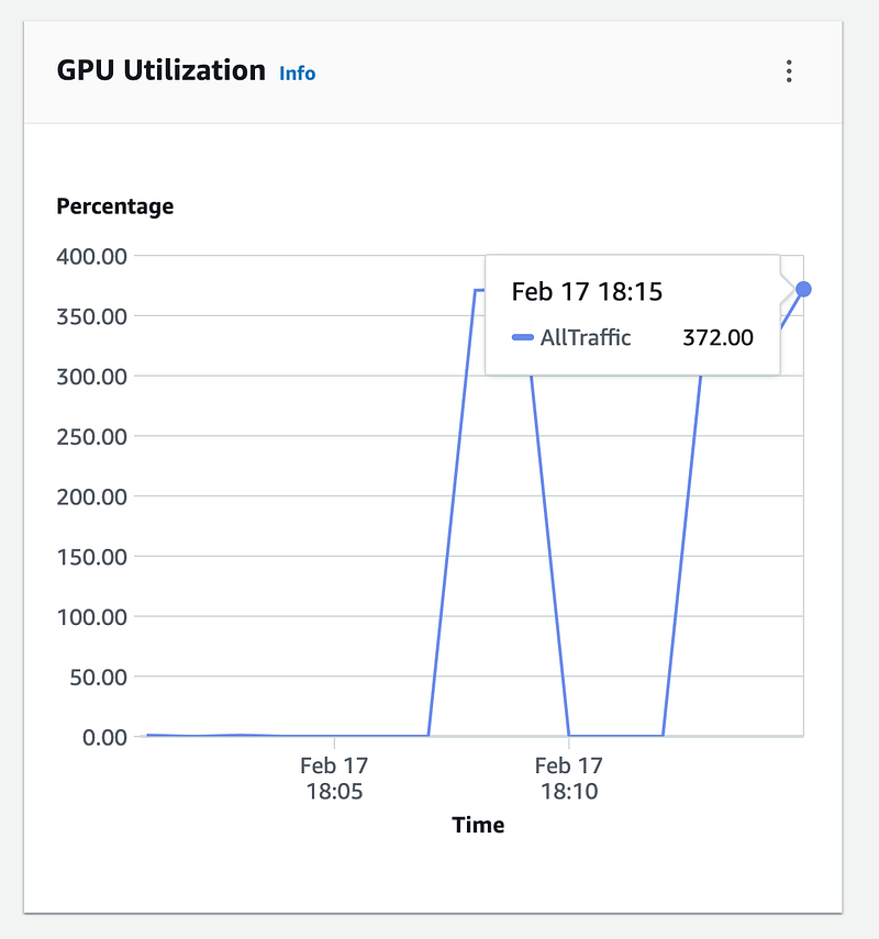
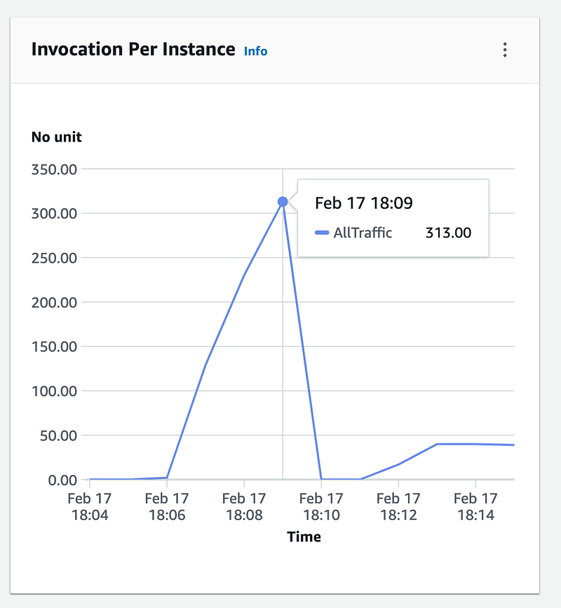
GPU Utilization (400% Available for 4 GPUs)

We see that we are able to saturate our hardware with our current load testing setup, giving us an idea of what our current configuration gives us performance wise for a singular instance. Note that you can tune this further by adjusting factors such as Batch Size, Quantization method, and more to arrive at your optimal configuration.

Optionally at the hardware level you can also define an AutoScaling policy. In this case we define an aggressive policy to scale out at five requests in a minute. You can define this scaling policy on the CloudWatch metric of your choice.

# AutoScaling client
asg = boto3.client('application-autoscaling')

# Resource type is variant and the unique identifier is the resource ID.
# default VariantName is AllTraffic adjust for your use-case
resource_id=f"endpoint/{predictor.endpoint_name}/variant/AllTraffic"

# scaling configuration
response = asg.register_scalable_target(
    ServiceNamespace='sagemaker', #
    ResourceId=resource_id,
    ScalableDimension='sagemaker:variant:DesiredInstanceCount', 
    MinCapacity=1,
    MaxCapacity=4
)

#Target Scaling
response = asg.put_scaling_policy(
    PolicyName=f'Request-ScalingPolicy-{endpoint_name}',
    ServiceNamespace='sagemaker',
    ResourceId=resource_id,
    ScalableDimension='sagemaker:variant:DesiredInstanceCount',
    PolicyType='TargetTrackingScaling',
    TargetTrackingScalingPolicyConfiguration={
        'TargetValue': 5.0, # Threshold, 5 requests in a minute
        'PredefinedMetricSpecification': {
            'PredefinedMetricType': 'SageMakerVariantInvocationsPerInstance',
        },
        'ScaleInCooldown': 300, # duration until scale in
        'ScaleOutCooldown': 60 # duration between scale out
    }
)

We send requests continuously for 15 minutes and can see our endpoint update to four instances as we have defined in our policy:

import time
request_duration = 60 * 15 # 15 minutes
end_time = time.time() + request_duration
print(f"test will run for {request_duration} seconds")
while time.time() < end_time:
    response = runtime_client.invoke_endpoint(
        EndpointName=endpoint_name,
        ContentType=content_type,
        Body=json.dumps(payload))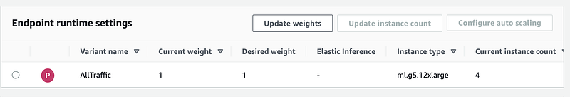

Scaled Up Endpoint (Screenshot by Author)

4. Additional Resources & Conclusion

SageMaker-Deployment/LLM-Hosting/DJL-Serving/Mistral7B at master · RamVegiraju/SageMaker-Deployment

Compilation of examples of SageMaker inference options and other features. …

github.com

The code for the entire article can be found at the link above. I hope this article was a useful guide for optimizing LLM deployment on SageMaker Real-Time Inference. A great guide that I utilized as a reference is the following Nvidia Blog which dives deeper into some of the concepts we have introduced today for LLM Inference. The LLM space is constantly changing and the rate of innovation has been incredible to say the least. Stay tuned for further articles in this space!

As always thank you for reading and feel free to leave any feedback.

If you enjoyed this article feel free to connect with me on LinkedIn and subscribe to my Medium Newsletter.