
(3) OPTIMIZATION: Partial Derivatives and Gradients for Multivariate Functions
Understanding the basics

In my previous article, we reviewed some concepts from calculus, namely what a first-order and second-order derivative tell us about a function and how to find a local minimum for a function.
' All these ' reviewed concepts are only valid for univariate calculus (functions with only one variable). However, these functions are not the most common in machine learning, where several features (variables) are used to build models. This way, we will learn in this article how the concepts from univariate calculus can be extended for multivariate calculus and applied to find the minima of multivariate functions.
Now consider the function:
f(x,y) = 3x² + 2y⁴
We can also use Python to see our function:
import matplotlib.pyplot as plt
import numpy as np

# Define the function
def f(x, y):
    return 3 * x ** 2 + 2 * y ** 4

# Create a 3D meshgrid
x = np.linspace(-5, 5, 100)
y = np.linspace(-5, 5, 100)
X, Y = np.meshgrid(x, y)
Z = f(X, Y)

# Create the 3D plot
fig = plt.figure()
ax = fig.add_subplot(projection='3d')
ax.plot_surface(X, Y, Z, cmap='coolwarm')

# Set the labels and title
ax.set_xlabel('X')
ax.set_ylabel('Y')
ax.set_zlabel('Z')
ax.set_title('f(x,y) = 3x**2 + 2y**4')

# Show the plot
plt.show()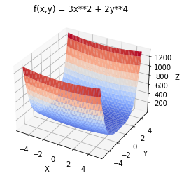
Partial derivative: A partial derivative is a derivative of a function in the order of one of its variables, while all other variables are held constant.
To find the partial derivatives of our function we apply the same rules as we use in univariate calculus: f’(x) = 6x f’(y) = 8y³
Gradient: We call a gradient the first derivative of a function with two or more variables. The gradient of an equation with n variables is a row vector with size 1xn, where each element is the partial derivative of f, concerning that variable:
f(x,y) = 3x² + 2y⁴
f’(x) = 6x f’(y) = 8y³
▽ f(x,y) = (6x, 8y³)
Let’s check:
#Get the partial derivatives:
#define x as a symbolic variable
x = sym.Symbol('x')
y = sym.Symbol('y')

#Define the function again as variable:
f_x = 3 * x ** 2
f_y = 2 * y ** 4

#Differentiate in order to x and y:
f_x_diff = sym.diff(f_x)
f_y_diff = sym.diff(f_y)
print('First order derivative of f(x) is: f´(x) =', f_x_diff)
print('First order derivative of f(y) is: f´(y) =', f_y_diff)
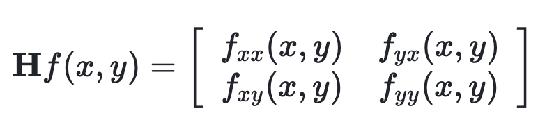
Hessian: Just as the first derivative of an equation with two or more variables has a special name (gradient), the second derivative also has a special name, Hessian, named after Ludwig Otto Hesse. And just as the gradient involves vectors formed from partial derivatives, the Hessian involves matrices. Let’s see…
→ Finding the second derivative of an equation with two or more variables, the Hessian, results in an nxn matrix, where each element is a partial derivative of the equation.
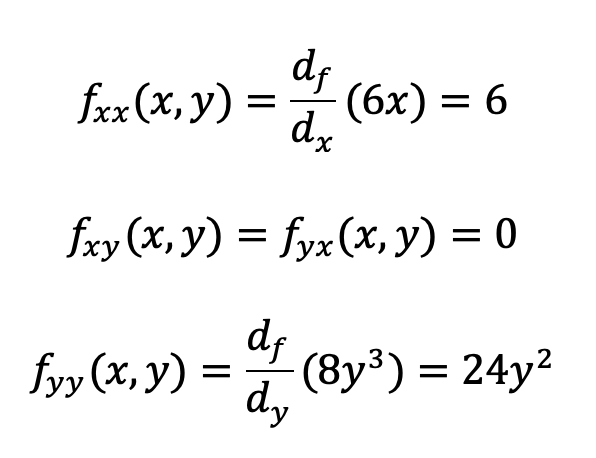
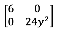
To get the Hessian for our equation:
f’’(x) = 6 f’’(y) = 24y⁴
And we can check our results using Python:
# Define the function
x, y = sym.symbols('x y')
f = 3*x**2 + 2*y**4

# Calculate the second partial derivatives
fx2 = sym.diff(f, x, 2)
fy2 = sym.diff(f, y, 2)
fxy = sym.diff(sym.diff(f, x), y)

# Construct the Hessian matrix
H = sym.Matrix([[fx2, fxy], [fxy, fy2]])

# Print the Hessian matrix
print("Hessian matrix:", H)
print('Second derivative f(x): ', fx2)
print('Second derivative f(y): ', fy2)
print('Second derivative f(x,y): ', fxy)
Now, if you haven’t read my previous articles on Linear algebra, it is time to do it!
Transpose of a matrix: Recall that the transpose of a matrix involves switching the rows and columns, such that the first row becomes that first column, the second row becomes the second column, and so on. If you transpose the Hessian matrix you will obtain exactly the same matrix. This phenomenon is called symmetry, and Hessian is always symmetric.
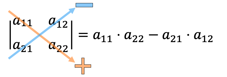
Determinant of a matrix: The determinant of the Hessian is also called the discriminant of f. For a two-variable function f(x, y) it is given y:
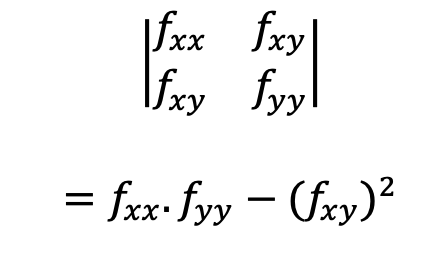
But as we have seen, Hessians are always symmetric, so it can be expressed as:
Using our previous example:
Determinant = 6 . 24y² — (0 . 0) = 144y²
We can also use Python to help us find the determinant:
# Find the determinant of the Hessian matrix
det_H = H.det()

# Print the determinant
print("Determinant of Hessian matrix:", det_H)
Now, let’s go a little bit further, and introduce eigenvectors and eigenvalues.
Eigenvector: When matrix A acts as a scaler multiplier on a vector X, then that vector is called the eigenvector of X. The value of the multiplier is known as the eigenvalue.
Eigenvalues for Hessians: → Because the Hessian of an equation is a square matrix, its eigenvalues can be found → Because Hessians are also symmetric, they have a special property that their eigenvalues will always be real numbers
The only thing we still need to worry about and find out, is if the eigenvalues are positive or negative!
Meaning of eigenvalues for Hessians: → Positive-definite matrix: If the Hessian at a given point has all positive eigenvalues, it is said to be a positive-definite matrix. This is the multivariable version of ‘concave up’ and is a SONC for a local minimum for the function f. → Negative-definite matrix: If all the eigenvalues are negative, it is said to be a negative-definite matrix. This is like ‘concave down’. → Saddle point: If the eigenvalues are mixed (positive and negative), we have a saddle point.
Now let’s go back to the determinant:
→ If det(Hessian) = 0, at a given point, then it means that there are zero eigenvalues, so we cannot make any conclusion. → If det(Hessian) < 0, at a given point, it means that eigenvalues have different signs, so we have a saddle point. → If det(Hessian) > 0, at a given point, it means that eigenvalues have the same sign, but we still don’t know if they are positive or negative.
We can try to find the value of the determinant at point (3,1):
144y² = 144.1 = 144 , so our eigenvalues have the same sign!
We can use the Trace of a Matrix to know if the sign is positive or negative!
→ If the trace is positive, means both values are positive → LOCAL MINIMUM! → If the trace is negative, means all values are negative → LOCAL MAXIMUM!
To find the trace of a matrix we sum the values of the main diagonal:
Trace = 6 + 24y² = 6 + 24(1) = 30, the value is positive, so the point (3, 1) meets the necessary conditions for a local minimum.
# Find the trace of the Hessian matrix
trace_H = H.trace()

# Print the trace
print("Trace of Hessian matrix:", trace_H)
Another way to find if a point is a candidate for a local minimum is to find the values for the eigenvalues. Let’s consider our Hessian matrix. To find the eigenvalues, the first step is to solve the following equation:
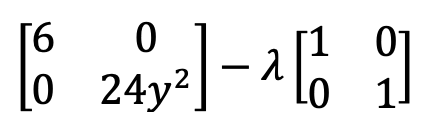
This is solved:
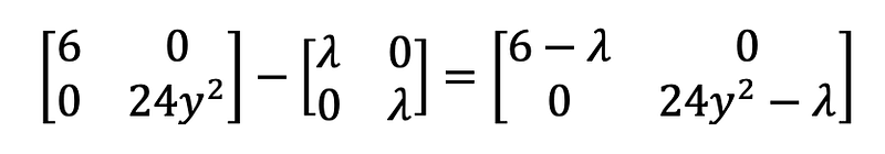
The next step is to find the determinant of the obtained matrix:
Determinant = 144y² — 6¥ — 24y²¥ + ¥²
Now we can try with the same point:
144 — 6¥ —24¥ + ¥² = ¥² — 30¥ + 144 ¥ = 6 and ¥ = 24
Both eigenvalues are positive, so our point meets the necessary conditions for a local minimum!
Conclusion The eigenvalues of the Hessian matrix will give us all we need to classify critical points. The determinant and trace are also useful but will hide the real eigenvalues. In this article, we applied these ideas to a function with two variables, but all we have learned also applies to functions from 2 to n variables, and the number of possible eigenvalues is the same as the number of variables in the equation. In the same way, the Hessian matrix you will obtain will be always a square matrix with the same size as the number of variables in your equation.
Thank you for reading! Don’t forget to subscribe to receive notifications about my future publications.
If: you liked this article, don’t forget to follow me and thus receive all updates about new publications.
Else If: you want to read more on the topic, you can buy my book “Data-Driven Decisions: A Practical Introduction to Machine Learning” which will give you all the information you need to start with Machine Learning. It will cost you only a coffee, and give me a small tip!
Else: Thank you!