
Optimization of Neural Networks with Linear Solvers
How to optimize nonlinear neural networks in more than one dimension using linear solvers.

Recently, I stumbled over a problem that required me to create a model which takes more than one input feature and predicts a continuous output.
Then, I needed to get the best possible output from that model, which in my case was the lowest possible numerical value. So, in other words, I needed to solve an optimization problem.
The issue was (and I only realized it at that stage) that the environment I was working in did not allow me to use nonlinear things or sophisticated frameworks— so no neural networks, no nonlinear solvers, nothing...
But, the model I created worked well (considering the low number of data points I trained it on), and I did not want to delete all my codes and start from scratch with a linear model.
So, after a cup of coffee ☕, I decided to use this nonlinear model I already trained to generate a number of small linear ones. Then I could use a linear solver to solve the optimization problem.
Sounds maybe not like the best or most promising idea, but at least it sounds exciting 😄.
This notebook is a step-by-step example of how this whole thing worked. So get a coffee ☕, start Python 🐍, and follow me 😄.
Initial idea to get a larger dataset
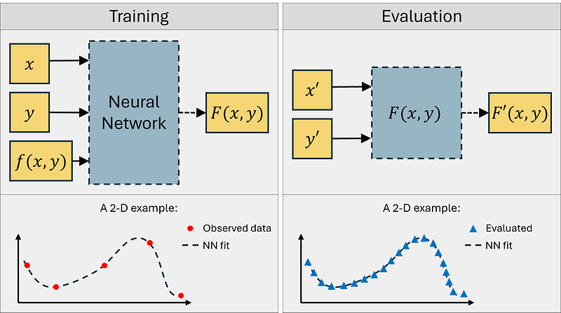
So, the initial steps I mentioned above are visualized in Figure 1.
We got some features x and y and could observe some outputs f(x,y) from the real world. The dataset we colleced was relatively small. Also, we did this sampling in the past and we are not able to collect more samples. If we want to find an optimum using directly these data points or a linear interpolation between them, we might get inaccurate results, so let’s use another method.
As mentioned, I used this small data set to train a model. Let us stick to an artificial neural network (ANN) here and describe the trained neural network as F(x,y). Then, we can use this model and evaluate it as many times as we want.
Let’s say we generate a large vector of x-samples (in Figure 1 described by x’) and a large vector of y-samples (in Figure 1 described by y’). With this, we somehow augmented our dataset we had in the beginning.
Let us do this right away in Python, in two dimensions. 🐍
Data generation
In this earlier article, we looked at how to generate a good tasting cup of coffee ☕️, with one input being the brewing time, another input being the particle size of the ground coffee, and the output being a rating how well the coffee tastes.
Let us use a similar case study using the input feature x as the brewing time and another input feature y as the particle size of the ground coffee beans. Now, let us here look at the bitterness of the coffee, f(x,y), which we try to minimize.
Assume our underlying ground truth system f(x,y) (so our bitterness-function) has approximately the following functional form:

We will use some scaling below in the Python script in order to adjust it a bit to our physical meaning of the inputs
In Python, we can create the data as follows:
# Get some packages
import numpy as np
import matplotlib.pyplot as plt

# Get some data in two dimensions
xlb = 10    # [s] Lower bound for the brewing time
xub = 60    # [s] Upper bound for the brewing time
ylb = 0.05  # [mm] Lower bound for the particle size of the ground coffee
yub = 2     # [mm] Upper bound for the particle size of the ground coffee
x = np.linspace(xlb, xub, 5)
y = np.linspace(ylb, yub, 5)
X, Y = np.meshgrid(x, y)

# Define the output for the meshgrid and also in functional form for later
f = (np.sin(X/(xub-xlb)*2*np.pi) + np.cos(Y/(yub-ylb)*2*np.pi) + 2) / 4
def f_func(x, y):
    return (np.sin(x/(xub-xlb)*2*np.pi) + np.cos(y/(yub-ylb)*2*np.pi) + 2) / 4

# Plot the data in 3D
fig = plt.figure()
ax = fig.add_subplot(111, projection='3d')
ax.plot_surface(X, Y, f, alpha=0.5)
ax.scatter(X, Y, f, color='r')
ax.set_xlabel('x = Brewing time [s]')
ax.set_ylabel('y = Particle size [mm]')
ax.set_zlabel('Bitterness')

# Make a video
fignumber = 2
figname = f'Figure_{fignumber}'
makevideo = True
video_angle_velocity = 5
if makevideo:
    # Save figure normally
    plt.savefig(f'./{figname}.png', dpi=150)
    # Rotate figure and save frames
    for angle in list(np.linspace(0,360,int(360/video_angle_velocity))):
        ax.view_init(30, angle)
        # plt.draw() # Only needed in non-interactive mode (.py file)
        # plt.pause(.001) # Only needed in non-interactive mode (.py file)
        plt.savefig(f'./Figures/{figname}_{angle}.png', dpi=150)
    frames = []
    import imageio
    for angle in list(np.linspace(0,360,int(360/video_angle_velocity))):
        image = imageio.v2.imread(f'./Figures/{figname}_{angle}.png')
        frames.append(image)
    imageio.mimsave(f'./Figures/{figname}_gif.gif', # output gif
                    frames,          # array of input frames
                    fps = 5)         # optional: frames per second
else:
    figname = f'Figure_{fignumber}'
    plt.savefig(f'./{figname}.png', dpi=600)
    plt.show()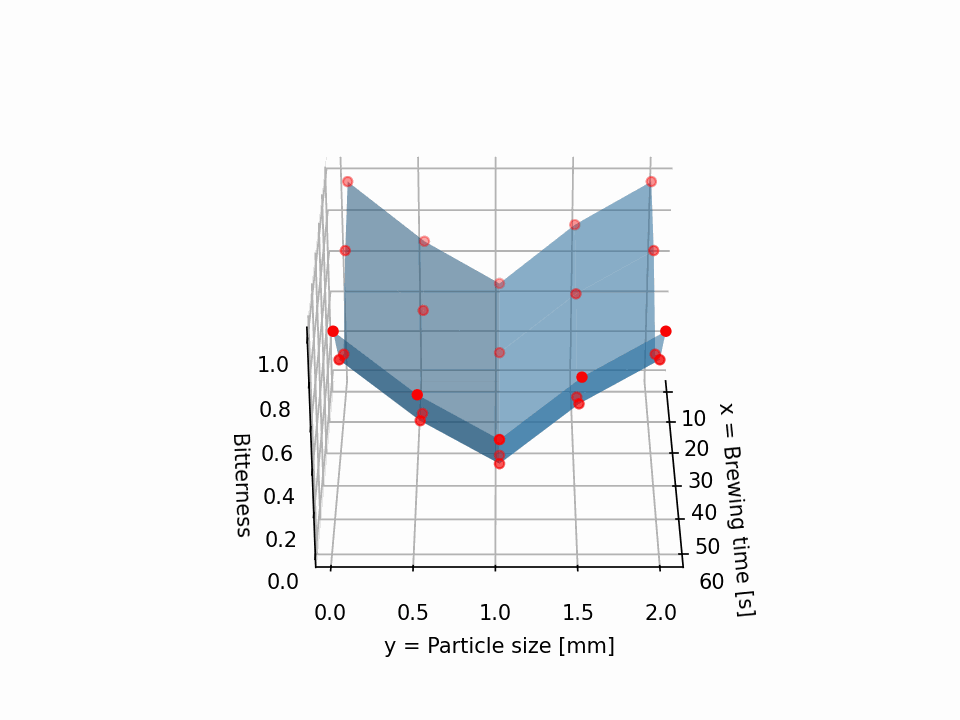
Model training
Next, let us train a neural network using the simple sklearn library. Since it does not matter, it’s fun, and because we can, we set up quite a large network 😄
In this tutorial, we will apply a feature scaling for the ANN. So let us also create a scaling function so that we do not have to write the whole thing over and over again:
# Train a neural network on the data X, Y and f
from sklearn.neural_network import MLPRegressor

# Scale the x and y data between 0 and 1
def xscale(x_):
    return (x_-xlb)/(xub-xlb)
def yscale(y_):
    return (y_-ylb)/(yub-ylb)
def xunscale(x_):
    return x_*(xub-xlb) + xlb
def yunscale(y_):
    return y_*(yub-ylb) + ylb

# Create meshgrid
X_ann, Y_ann = np.meshgrid(xscale(x), yscale(y))

# Train the neural network
ANN = MLPRegressor(hidden_layer_sizes=(100,100,100), max_iter=1000, random_state=0)
ANN.fit(np.c_[X_ann.ravel(), Y_ann.ravel()], f.ravel())

# Evalaute the ANN at the given datapoints
F = ANN.predict(np.c_[X_ann.ravel(), Y_ann.ravel()]).reshape(X_ann.shape)
Now we have our trained (and probably overpowerd) neural network F(x,y). Cool! 😎
As shown in Figure 1, we can evaluate this network at arbitrarily many points in the x-y-plane (remember to scale the data).
Before we only had 5 points per dimension, so let us use much more now:
# Create new arbitrary points for our x- and y-axes
nevalpoints = 80
x_eval_unscaled = np.linspace(xlb, xub, nevalpoints)
y_eval_unscaled = np.linspace(ylb, yub, nevalpoints)
X_eval_unscaled, Y_eval_unscaled = np.meshgrid(x_eval_unscaled, y_eval_unscaled)

# Scale the new points
x_eval = xscale(x_eval_unscaled)
y_eval = yscale(y_eval_unscaled)
X_eval, Y_eval = np.meshgrid(x_eval, y_eval)

# Evaluate the neural network on these points
F_eval = ANN.predict(np.c_[X_eval.ravel(), Y_eval.ravel()]).reshape(X_eval.shape)
Finally, we can visualize all the things we did:
# Create 3D figures
fig = plt.figure(figsize=(10,5))
# Since all 3D plots are the same, we can use a function to create them
def plot_3d(ax, X_, Y_, Z_, title):
ax.plot_surface(X_, Y_, Z_, cmap='viridis', edgecolor='none')
ax.scatter(X, Y, f, color='r')
ax.set_xlabel('$x$')
ax.set_xticks(np.linspace(xlb, xub, 3).astype('int'))
ax.set_ylabel('$y$')
ax.set_yticks(np.linspace(ylb, yub, 3).astype('int'))
ax.set_zticks(np.linspace(0, 1, 3).astype('int'))
ax.set_title(title)
# Plot the data in 3D
ax1 = fig.add_subplot(131, projection='3d')
plot_3d(ax1, X, Y, f, 'Data - $f(x,y)$')
# Plot the neural network in 3D
ax2 = fig.add_subplot(132, projection='3d')
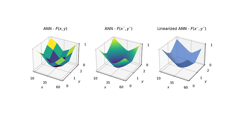
plot_3d(ax2, X, Y, F, 'ANN - $F(x,y)$')
# Evaluate the neural network at more points and plot in 3D
ax3 = fig.add_subplot(133, projection='3d')
plot_3d(ax3, X_eval_unscaled, Y_eval_unscaled, F_eval, 'ANN evaluated - $F(x´,y´)$')
# Save the figure
fignumber += 1
figname = f'Figure_{fignumber}'
plt.savefig(f'./{figname}.png', dpi=600)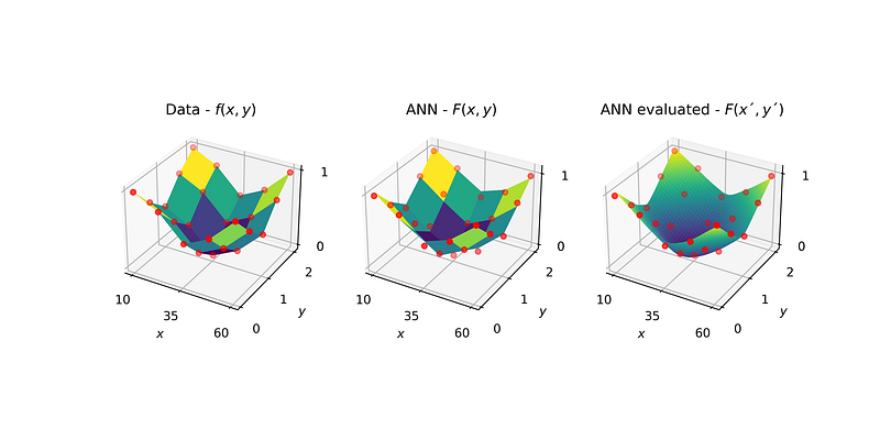
Now we have a model F(x,y) for our system f(x,y) and we have available many more data points than in the beginning. Looks smoother, doesn’t it? This is the concept we are gonna use. 😃
We would like to linearize the model in a next step. And for a linearization, having more data points available is definitely an andvantate since we can better capture curvature and nonlinearities (since we approximate the ANN that is nonlinear) over the entire space (but still not between the individual points of course).
Linearization in two dimensions
In an earlier article, I described how to linearize a model in one dimension:
As mentioned, we will do the same now, but in two dimensions.
Linearizations with one feature (only x) results in a line. Linearization with two features (x and y) results in a plane. So, let us grab the linear equation for a plane:

In this expression, a and b are the slopes of the plane (in the x- and y-direction), and c is a constant. As an approximation, the slopes a and b can be found by using the finite difference method:

where delta-x and delta-y are small steps in the x and y directions, respectively.
Let us plug that back into the linear equation for the plane:

Cool, so we have (in almost-a-bit-scary-looking mathy theory) a possibility to linearize something in two dimensions.
To draw a line, in general, we need two points. To draw a plane, however, we need one more (we have three unknown coefficients, a,b, and c, so we need three equations and therefore three data points). In mathematical terms:

We can rearrange these equations in order to calculate the slopes and intersections:

Now, get a sip of your coffee ☕ and then we implement everything in Python 😊🐍
Piecewise linearization in two dimensions
So, we do not only want to create a plane from one end of our space to the other end. We can split our entire space into as many small segments as we wish and then draw such a plane for each segment.
First, let us create these segments in x and y directions, which I will describe by indices i and j.
So, now we can create a function that calculates the coefficients a, b, and c for a plane, given the points x1, x2, y1, y2, f1, f2, and f3 (which are basically the edge points of our created segments):
# In order to get the slopes (in x- and y-direction) and the intersection, we need three points (x1,y1), (x1,y2), and (x2,y1)
# with these points we can solve the system of equations to get the slopes a, b, and the intersection c
# The linear function is then f(x,y) = a*x + b*y + c
def calc_slopes_and_intersection(x1,x2,y1,y2,f1,f2,f3):
    # Calculate the slopes
    a = (f2 - f1)/(x2 - x1)
    b = (f3 - f1)/(y2 - y1)
    # Calculate the intersection
    c = f1 - a*x1 - b*y1
    return a, b, c

# Define a function that outputs the linear function for a given segment
def get_linear(x1,x2,y1,y2,f1,f2,f3):
    # With the given two points for each dimension, we calculate the equation of the plane
    a, b, c = calc_slopes_and_intersection(x1,x2,y1,y2,f1,f2,f3)
    # Calculate linear approximation value at the given point
    lin_approx = a*x1 + b*y1 + c
    # Print the linear function to the console
    print(f'[+] Linear function for segment of x=[x1,x2]=[{x1:.1f},{x2:.1f}] and y=[y1,y2]=[{y1:.1f},{y2:.1f}]: f={a:.1f}*x + {b:.1f}*y + {c:.1f}')
    return lin_approx, a,b,c
Now we need to be able to evaluate the neural network we trained at the points x1, x2, y1, and y2. We can do this by creating a nicer function:
def evaluate_neural_network(x__, y__):
    # Returns the predicted value of the neural network at the given point
    # Remember to scale the inputs
    x__ = xscale(x__)
    y__ = yscale(y__)
    F_point_eval = ANN.predict(np.c_[x__.ravel(), y__.ravel()]).reshape(x__.shape)
    return F_point_eval
Let us look at a comparison if we use a small number of segments and our original neural network (I mean, the neural network we trained on only a small number of data points). We can then plot the underlying system and our linearized ANN:
# To linearize the neural network, we need to create segments in two dimensions
# We will create a grid of segments
num_x_segments = 5
num_y_segments = 5
x_segments = np.linspace(xlb, xub, num_x_segments+1)
y_segments = np.linspace(ylb, yub, num_y_segments+1)

# Calculate the linear functions for each segment
a_list = np.zeros((num_x_segments, num_y_segments))
b_list = np.zeros((num_x_segments, num_y_segments))
c_list = np.zeros((num_x_segments, num_y_segments))
F_lin = np.zeros((num_x_segments, num_y_segments))
for i in range(num_x_segments):
    for j in range(num_y_segments):
        # Get points in x direction
        x1 = x_segments[i]
        x2 = x_segments[i+1]
        # Get points in y direction
        y1 = y_segments[j]
        y2 = y_segments[j+1]
        # Get the z values for the four points
        z1 = evaluate_neural_network(x1,y1)
        z2 = evaluate_neural_network(x2,y1)
        z3 = evaluate_neural_network(x1,y2)
        # Calculate the linear function
        F_lin[j,i], a_,b_,c_ = get_linear(x1,x2, y1,y2, z1,z2,z3)
        # Append slopes and intersection
        a_list[j,i] = a_
        b_list[j,i] = b_
        c_list[j,i] = c_

# Get the figure
X_seg_small, Y_seg_small = np.meshgrid(x_segments[:-1], y_segments[:-1])
fig = plt.figure()

# Plot the ANN
ax = fig.add_subplot(111, projection='3d')
ax.plot_surface(X, Y, f, cmap='viridis', edgecolor='none', alpha=0.5)
ax.plot_surface(X_seg_small, Y_seg_small, F_lin, color='red', edgecolor='black', alpha=0.8)
ax.set_xlabel('$x$')
ax.set_ylabel('$y$')

# Save the figure
fignumber += 1
figname = f'Figure_{fignumber}'
plt.savefig(f'./{figname}.png', dpi=600)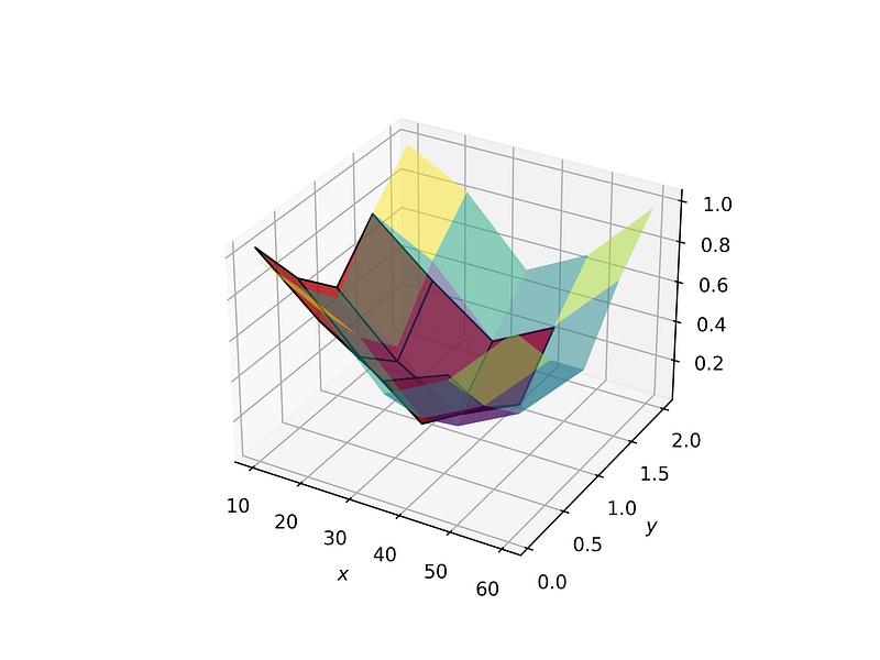
So, this somehow works, just that we use planes for quite a big part of the entire space (too little number of segments).
Also, quite a bit of the space is not approximated. This is of course because we always need two points in each dimension (i.e., x1 and x2) to create one plane, meaning for n points we only get n-1 planes. So for the last segment, we cannot create a plane since we would need an x value that is out of our considered space. Let us switch back to a looot of segments and visualize the result:
Use the same code snipped for the number of segments and just change it to a large number.
# To linearize the neural network, we need to create segments in two dimensions
# We will create a grid of segments
num_x_segments = 15
num_y_segments = 15
x_segments = np.linspace(xlb, xub, num_x_segments+1)
y_segments = np.linspace(ylb, yub, num_y_segments+1)

# Calculate the linear functions for each segment
a_list = np.zeros((num_x_segments, num_y_segments))
b_list = np.zeros((num_x_segments, num_y_segments))
c_list = np.zeros((num_x_segments, num_y_segments))
F_lin = np.zeros((num_x_segments, num_y_segments))
for i in range(num_x_segments):
    for j in range(num_y_segments):
        # Get points in x direction
        x1 = x_segments[i]
        x2 = x_segments[i+1]
        # Get points in y direction
        y1 = y_segments[j]
        y2 = y_segments[j+1]
        # Get the z values for the four points
        z1 = evaluate_neural_network(x1,y1)
        z2 = evaluate_neural_network(x2,y1)
        z3 = evaluate_neural_network(x1,y2)
        # Calculate the linear function
        F_lin[j,i], a_,b_,c_ = get_linear(x1,x2, y1,y2, z1,z2,z3)
        # Append slopes and intersection
        a_list[j,i] = a_
        b_list[j,i] = b_
        c_list[j,i] = c_

# Get the figure
X_seg_large, Y_seg_large = np.meshgrid(x_segments[:-1], y_segments[:-1])
fig = plt.figure(figsize=(10,5))

# Since the plots are the same, let's define a function for them
def plot_3d(ax, X_, Y_, Z_, title, color=None):
    if color is not None:
        ax.plot_surface(X_, Y_, Z_, color=color, edgecolor='none', alpha=0.8)
    else:
        ax.plot_surface(X_, Y_, Z_, cmap='viridis', edgecolor='none', alpha=1)
    ax.set_xlabel('$x$')
    ax.set_xticks(np.linspace(xlb, xub, 3).astype('int'))
    ax.set_ylabel('$y$')
    ax.set_yticks(np.linspace(ylb, yub, 3).astype('int'))
    ax.set_zticks(np.linspace(0, 1, 3).astype('int'))
    ax.set_title(title)

# Plot the ANN
ax = fig.add_subplot(131, projection='3d')
plot_3d(ax, X, Y, f, 'ANN - $F(x,y)$')

# Plot the evaluated ANN
ax = fig.add_subplot(132, projection='3d')
plot_3d(ax, X_eval_unscaled, Y_eval_unscaled, F_eval, 'ANN - $F(x´,y´)$')

# Plot the linearization
ax = fig.add_subplot(133, projection='3d')
plot_3d(ax, X_seg_large, Y_seg_large, F_lin, 'Linearized ANN - $F(x´,y´)$', color='cornflowerblue')

# Save the figure
fignumber += 1
figname = f'Figure_{fignumber}'
plt.savefig(f'./{figname}.png', dpi=600)[+] Linear function for segment of x=[x1,x2]=[10.0,13.3] and y=[y1,y2]=[0.1,0.2]: f=-0.0*x + -0.5*y + 1.2
[+] Linear function for segment of x=[x1,x2]=[10.0,13.3] and y=[y1,y2]=[0.2,0.3]: f=-0.0*x + -0.6*y + 1.3
[+] Linear function for segment of x=[x1,x2]=[10.0,13.3] and y=[y1,y2]=[0.3,0.4]: f=-0.0*x + -0.6*y + 1.3
[+] Linear function for segment of x=[x1,x2]=[10.0,13.3] and y=[y1,y2]=[0.4,0.6]: f=-0.0*x + -0.6*y + 1.3
[+] Linear function for segment of x=[x1,x2]=[10.0,13.3] and y=[y1,y2]=[0.6,0.7]: f=-0.0*x + -0.5*y + 1.3
[+] Linear function for segment of x=[x1,x2]=[10.0,13.3] and y=[y1,y2]=[0.7,0.8]: f=-0.0*x + -0.4*y + 1.2
[+] Linear function for segment of x=[x1,x2]=[10.0,13.3] and y=[y1,y2]=[0.8,1.0]: f=-0.0*x + -0.3*y + 1.2
[+] Linear function for segment of x=[x1,x2]=[10.0,13.3] and y=[y1,y2]=[1.0,1.1]: f=-0.0*x + -0.0*y + 0.9
[+] Linear function for segment of x=[x1,x2]=[10.0,13.3] and y=[y1,y2]=[1.1,1.2]: f=-0.0*x + 0.4*y + 0.3
...
Cool, so now we have approximated our nonlinear neural network (with also more or less the same accuracy) with linear functions.
This allows us to go back to our original problem and plug our “neural network” into an optimization problem. Before jumping to Pyomo, let us first define our optimization problem on paper (or your screen 😄).
Optimization
From this point onwards we follow a very similar path as described in one of my earlier articles:
Let us first define the optimization problem of our real system f(x,y). We can write the problem as follows:

Let us say we do not have any constraints (so no g(x,y)), so we can just minimize our function, so we get:

Now what we first did is replaced our real system f(x,y) by our neural network F(x,y), so the problem now reads:

Further, we then generated our linear approximation for F(x,y). If we would do one single plane for our approximation, the problem would read as follows:

However, we used several planes, not only one. So we need to consider all of them, which we do by giving each plane the index i (in x direction) and j (in y direction). Also, since our solution can only be in one segment at the time, we need to be able to activate and deactivate the segments. We do this by introducing a binary variable z for each segment ij. This variable is 1 if our solution (x,y) is in the segment, and 0 otherwise. Since the solution can only be in one segment at the time, all z-values need to sum up to 1. Now our problem reads a follows:

Or in another notation:

The issue with this notation is that the objective function is still nonlinear (due to the multiplication of x with z and y with z in the objective function). We call a multiplication of a binary variable (z) with a continuous variable (x) “pseudo bilinear”. We can use a cool trick that allows us rewriting such a pseudo bilinear term. First, we define two auxiliary variables alpha and beta, which are the multiplications of the continuous variables (x and y) with the binary variable (z):

Next, we need to define the validity for alpha and beta for the cases when z=0 (inactive segment) and z=1 (active segment). If the segment is inactive, our auxiliary variables needs to be zero. We achieve this by the following inequalities:

Where xmin and xmax are the lower- and upper ends of our segments which we calculated above. You can easily verify that if z is zero, alpha or beta is forced to be zero as well.
In addition, if z=1, the auxilary variables alpha or beta should be bounded by the “true” continuous variables x and y:

It is worth to mention here that x/y-upper are the upper bounds of the continuous variables x and y (not the ones of the segments). With this, we can rewrite our final optimization problem from above:

Now with this, we are done. Maybe take a sip of your tasty coffee first ☕ and then let us implement this in Python using the Pyomo library.
Pyomo implementation
First, we import Pyomo itself and then we create a concrete model:
import pyomo.environ as pyo
objmodel = pyo.ConcreteModel()
Then, we define the sets I and J (the segments in x and y direction), the continuous variables x,y, alpha and beta, and the binary variable z. In addition, we initialize them in an appropriate manner (many possibilities):
# Define the set of segments
I = range(num_x_segments)
J = range(num_y_segments)
objmodel.I = pyo.Set(initialize=I)
objmodel.J = pyo.Set(initialize=J)

# Define the continuous variable
objmodel.x = pyo.Var(initialize = xlb, bounds = (xlb, xub), domain=pyo.Reals)
objmodel.y = pyo.Var(initialize = ylb, bounds = (ylb, yub), domain=pyo.Reals)

# Define the auxiliary continuous variables
def alpha_bounds(m,i,j):
    lb = 0
    ub = xub
    return (lb, ub)
def beta_bounds(m,i,j):
    lb = 0
    ub = yub
    return (lb, ub)
def alpha_init(m,i,j):
    return x_segments[i]
def beta_init(m,i,j):
    return y_segments[j]
objmodel.alpha = pyo.Var(objmodel.I, objmodel.J, initialize = alpha_init, bounds = alpha_bounds, domain=pyo.Reals)
objmodel.beta = pyo.Var(objmodel.I, objmodel.J, initialize = beta_init, bounds = beta_bounds, domain=pyo.Reals)

# Define the binary variables
def z_init(m,i,j):
    if i == 0 and j == 0:
        return 1
    else:
        return 0
objmodel.z = pyo.Var(objmodel.I, objmodel.J, initialize=z_init, domain=pyo.Binary)
The next step is the definition of the objective function, which we would like to minimize (check that the indices settings for the slopes and intersections are correct):
objmodel.obj = pyo.Objective(expr = sum([sum([(a_list[j,i]*objmodel.alpha[i,j] + b_list[j,i]*objmodel.beta[i,j] + c_list[j,i]*objmodel.z[i,j]) for i in objmodel.I]) for j in objmodel.J]), sense=pyo.minimize)In addition, we need our constraints, which we can define with rules or expressions. First, the summation of all our binary variables:
objmodel.c1 = pyo.Constraint(expr = sum([sum([objmodel.z[i,j] for i in objmodel.I]) for j in objmodel.J]) == 1)Next, our constraints to transform the bilinear terms:
# Define rules for the constraints that transform the bilinear term for x
def c2_rule(m, i, j):
    xmin = x_segments[i]
    return xmin*m.z[i,j] <= m.alpha[i,j]
def c3_rule(m, i, j):
    xmax = x_segments[i+1]
    return m.alpha[i,j] <= xmax*m.z[i,j]
def c4_rule(m, i, j):
    return m.x - xub*(1-m.z[i,j]) <= m.alpha[i,j]
def c5_rule(m, i, j):
    return m.alpha[i,j] <= m.x

# Define rules for the constraints that transform the bilinear term for y
def c6_rule(m, i, j):
    ymin = y_segments[j]
    return ymin*m.z[i,j] <= m.beta[i,j]
def c7_rule(m, i, j):
    ymax = y_segments[j+1]
    return m.beta[i,j] <= ymax*m.z[i,j]
def c8_rule(m, i, j):
    return m.y - yub*(1-m.z[i,j]) <= m.beta[i,j]
def c9_rule(m, i, j):
    return m.beta[i,j] <= m.y

# Use the rules to write the constraints
objmodel.c2 = pyo.Constraint(objmodel.I, objmodel.J, rule = c2_rule)
objmodel.c3 = pyo.Constraint(objmodel.I, objmodel.J, rule = c3_rule)
objmodel.c4 = pyo.Constraint(objmodel.I, objmodel.J, rule = c4_rule)
objmodel.c5 = pyo.Constraint(objmodel.I, objmodel.J, rule = c5_rule)
objmodel.c6 = pyo.Constraint(objmodel.I, objmodel.J, rule = c6_rule)
objmodel.c7 = pyo.Constraint(objmodel.I, objmodel.J, rule = c7_rule)
objmodel.c8 = pyo.Constraint(objmodel.I, objmodel.J, rule = c8_rule)
objmodel.c9 = pyo.Constraint(objmodel.I, objmodel.J, rule = c9_rule)
Now, that’s it! We have defined our optimization problem. We can now solve it using a solver. In this case, we use the open-source solver GLPK (a linear solver), since our problem is fully linear:
# Solve the model
solver = pyo.SolverFactory('glpk')
results = solver.solve(objmodel)
The results can be stored and extracted in order to print the results to the console (since the solver sometimes gives back very small numbers instead of zero, we use a “cutoff-threshold”):
# Write the relevant things to variables
threshold = 1e-6
optobj = objmodel.obj()
optalpha = [objmodel.alpha[i,j]() if objmodel.alpha[i,j]() >= threshold else 0 for i in objmodel.I for j in objmodel.J]
optbeta = [objmodel.beta[i,j]() if objmodel.beta[i,j]() >= threshold else 0 for i in objmodel.I for j in objmodel.J]

# Extract non-zero elements
from itertools import compress
nonzero_index_alpha = list(compress(range(len(optalpha)), optalpha))
nonzero_index_beta = list(compress(range(len(optbeta)), optbeta))

# Get solver status
print(f'[+] Solver status: {results.solver.status}')
print(f'[+] Solver termination condition: {results.solver.termination_condition}')

# Print results
print(f'[+] Optimal objective value: {optobj:.3f}')
print(f'[+] Optimal x value: {objmodel.x():.3f}')
print(f'[+] Optimal y value: {objmodel.y():.3f}')
print(f'[+] Optimal alpha value: {optalpha[nonzero_index_alpha[0]]:.3f}')
print(f'[+] Optimal beta values: {optbeta[nonzero_index_beta[0]]:.3f}')
[+] Solver status: ok
[+] Solver termination condition: optimal
[+] Optimal objective value: 0.077
[+] Optimal x value: 36.667
[+] Optimal y value: 0.960
[+] Optimal alpha value: 36.667
[+] Optimal beta values: 0.960And finally, we can visualize the results which is always the best part 😄
# Create 3D figures
fig = plt.figure(figsize=(10,5))

# Plot the data in 3D
ax = fig.add_subplot(111, projection='3d')
ax.plot_surface(X, Y, f, cmap='viridis', edgecolor='none', alpha=0.7)       # Underlying data
ax.plot_surface(X_seg_large, Y_seg_large, F_lin, color='blue', edgecolor='black', alpha=0.5)   # Linearized ANN
ax.scatter(objmodel.x(), objmodel.y(), optobj, marker = 'd', color='blue', s=100, label='Model Optimum')
ax.set_xlabel('$x$')
ax.set_ylabel('$y$')

# Make a video
fignumber += 1
figname = f'Figure_{fignumber}'
makevideo = True
video_angle_velocity = 5
if makevideo:
    # Save figure normally
    plt.savefig(f'./{figname}.png', dpi=150)
    # Rotate figure and save frames
    for angle in list(np.linspace(0,360,int(360/video_angle_velocity))):
        ax.view_init(30, angle)
        # plt.draw() # Only needed in non-interactive mode (.py file)
        # plt.pause(.001) # Only needed in non-interactive mode (.py file)
        plt.savefig(f'./Figures/{figname}_{angle}.png', dpi=150)
    frames = []
    import imageio
    for angle in list(np.linspace(0,360,int(360/video_angle_velocity))):
        image = imageio.v2.imread(f'./Figures/{figname}_{angle}.png')
        frames.append(image)
    imageio.mimsave(f'./Figures/{figname}_gif.gif', # output gif
                    frames,          # array of input frames
                    fps = 5)         # optional: frames per second
else:
    plt.savefig(f'./{figname}.png', dpi=600)
    plt.show()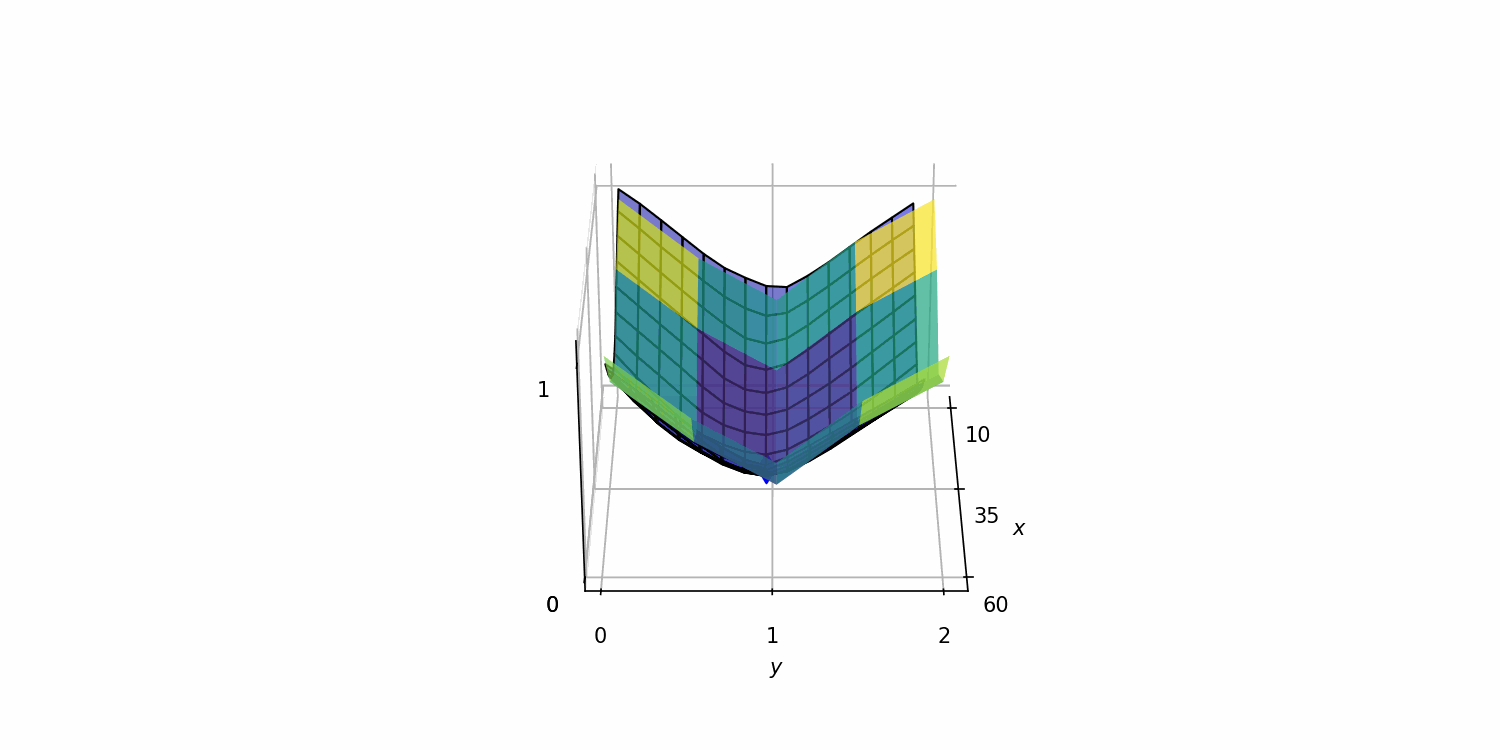
Or in a 2D projection:
# Get the figure
fig = plt.figure()

# Plot the data in the x-y-plane
ax = fig.add_subplot(111)
ax.contourf(X, Y, f, cmap='viridis', alpha=0.8)                         # Underlying data

# Add a color bar for the real data
cbar = plt.colorbar(ax.contourf(X, Y, f, cmap='viridis', alpha=0.8))
cbar.set_label('$f(x,y)$')

# Add the rest of the data
ax.contour(X_seg_large, Y_seg_large, F_lin, colors='black', alpha=1)    # Linearized ANN
ax.scatter(objmodel.x(), objmodel.y(), marker = 'o', color='red', s=100, label='Model Optimum')
ax.set_xlabel('$x$')
ax.set_ylabel('$y$')
ax.legend()

# Save the figure
fignumber += 1
figname = f'Figure_{fignumber}'
plt.savefig(f'./{figname}.png', dpi=600)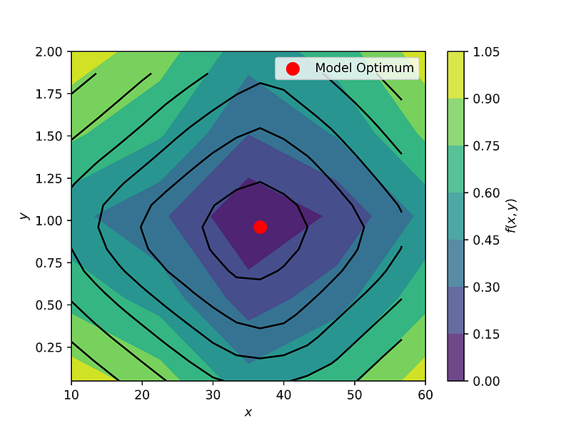
Nice, so we used planes to approximately find the optimum in two dimensions, although we only had very little number of data points in the beginning. 😎
So, tune your coffee bean grinder to a particle size of around y = 1 mm and brew the coffee for around x = 37 seconds to reach the lowest bitterness — which is very close to the true optimum, as we see in the figure above! ☕️
Conclusion
That was it! So we went through quite a lot of topics today. We started with a nonlinear neural network that was trained on only a few data points, and which we then approximated with many planes (instead of approximating the small data set with those planes). We then used this linear approximation to solve an optimization problem to find the settings for a good coffee.
I hope you enjoyed this article and that you learned something new, I definitely did! 😄 If you liked it, hit the clap button (the optimum is located at infinitely many times, assuming no constraints 😄) and maybe check out my other articles:
Thanks for reading and happy optimizing! ☕😄🐍


