
OpenCV: Count of Objects in Blood Image with Python
Image processing concept with OpenCV library
In this article, we will discuss object segmentation with the help of the OpenCV library and pre-processing techniques in image processing. We will try to mark the contours with the number to get the total number of objects.
What is OpenCV?
It is an open-source library to process images and videos for various applications in real life, like segmentation, object detection, and many more. The main benefit of the OpenCV library is working on NumPy arrays that can be work with a different library.
The process to count the objects in an image is done with the below process:
Step1: Importing the libraries and reading the input image with the help of these libraries.
Importing the necessary libraries
import numpy as np
import imutils
import cv2
The “numpy” library is an open-source that contains data in multi-dimensional and matrix array form and processing these array data. The “imutils” is used to manipulate the image with basic functions like rotation, resizing, etc. The “cv2” is a computer vision library.
Reading the input image of blood object.
image = cv2.imread('blood.jpg') #reads the image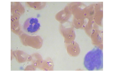
Step 2: Using De-noising and Blur filters to get a more clear image for processing.
We used a de-noising technique to remove the noise from the raw image for further processing. The de-noise is an image pre-processing process in computer vision.
dst = cv2.fastNlMeansDenoisingColored(image, None, 10, 10, 7, 15)#the meaning of parameters given
p1 = 10: size of pixels to compute weights of the image
p2 = 10: to compute the weighted average
p3 = 7: filter strength for luminescence
p4 = 15: filter strength for color componentWhen we read images in OpenCV it reads in BGR format and we need to change in RGB format for further processes.
rgb_image = cv2.cvtColor(dst, cv2.COLOR_BGR2RGB)we can also save the image with the imwrite function as shown below:
cv2.imwrite(‘RGB_image.jpg’,rgb_image)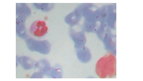
Now, we will use the median blur function to remove the salt-and-pepper noise. T working of this median blur to take the median of the filter window and replace the center pixel value with the median value pixel.
new_image = cv2.medianBlur(rgb_image,5)
cv2.imwrite('median_blur.jpg',new_image)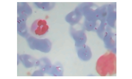
Latest Programming Languages for AI
Languages for AI to entertain it in the future
pub.towardsai.net
Step 3: Converting and Splitting of image into different color spaces
We have to convert the image into a particular color space to know the different channel of that color space. Here, we are taking a HSV color space and splitting in H,S and V channel.
hsv_image = cv2.cvtColor(new_image, cv2.COLOR_RGB2HSV)
h, s, v = cv2.split(hsv_image)
cv2.imwrite(‘H.jpg’,h)The view of the Different channels is shown below:
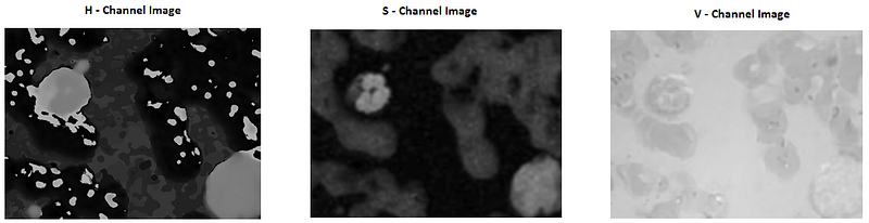
Step 4: Threshold the H — Channel image for binary image
This step is an important step to choose the perfect image to get to be a binary image for object detection. In the above images, we see that H — Channel image shows a pretty good sign to be a binary image because the pixel can be differentiating into two classes.
ret,th1=cv2.threshold(h,180,255, cv2.THRESH_BINARY+cv2.THRESH_OTSU)
cv2.imwrite('Binary_image.jpg',th1)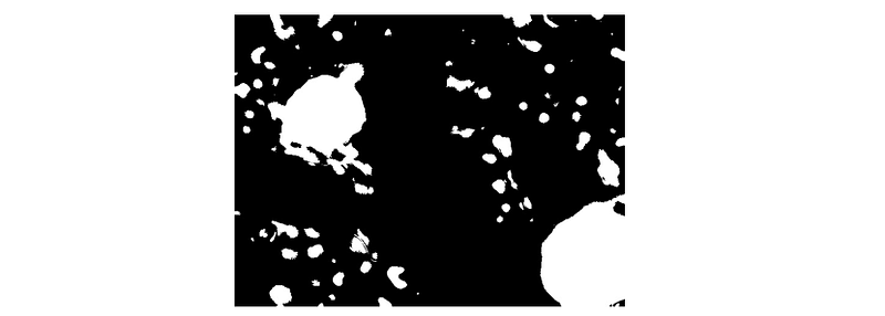
Now, we want the red object in the RGB image, so we try to use the morphological operation to reduce the noise.
kernel = np.ones((5,5), dtype = "uint8")/9
bilateral = cv2.bilateralFilter(th1, 9 , 75, 75)
erosion = cv2.erode(bilateral, kernel, iterations = 6)cv2.imwrite('mask_erosion.jpg', erosion)Here, we use the erode function to reduce the small white noise pixels from the binary image.

If you want to use the different method to remove the noise then check this article below:
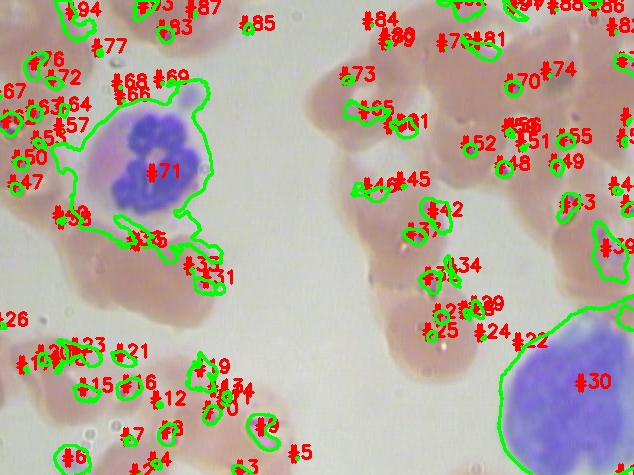
Step 5: To find the number of objects in the image and draw contour
In this step we try to draw the boundary or contour on the object and finding the total number of objects in the image.
# find contours in the thresholded image
cnts = cv2.findContours(th1.copy(), cv2.RETR_EXTERNAL,
 cv2.CHAIN_APPROX_SIMPLE)
cnts = imutils.grab_contours(cnts)
print("[INFO] {} unique contours found".format(len(cnts)))
#output:
[INFO] 6 unique contours found# loop over the contours
for (i, c) in enumerate(cnts):
# draw the contour
((x, y), _) = cv2.minEnclosingCircle(c)
cv2.putText(image, "#{}".format(i + 1), (int(x) - 10, int(y)),
cv2.FONT_HERSHEY_SIMPLEX, 0.6, (0, 0, 255), 2)
cv2.drawContours(image, [c], -1, (0, 255, 0), 2)
# show the output image
cv2.imshow("Image", image)
cv2.waitKey(0)cv2.imwrite('Contour_Image.jpg',image)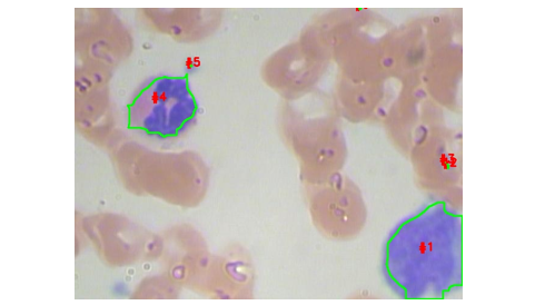
Conclusion
This article will give you a basic overview of the image pre-processing techniques.
I hope you like the article. Reach me on my LinkedIn and twitter.
Recommended Articles
1. NLP — Zero to Hero with Python 2. NumPy: Linear Algebra on Images 3. Exception Handling Concepts in Python 4. Principal Component Analysis in Dimensionality Reduction with Python 5. Fully Explained K-means Clustering with Python 6. Fully Explained Linear Regression with Python 7. Fully Explained Logistic Regression with Python 8. Differences Between concat(), merge() and join() with Python 9. Data Wrangling With Python — Part 1 10. Confusion Matrix in Machine Learning


