One of the Best Trend-Following Strategies

Creating a Strategy Based on the SuperTrend Pull-Back

The SuperTrend is a wonderful indicator that gives rise to many opportunities of strategies. Trend-following is a complex method that looks simple on books but needs a lot of care. This article discusses the flat pull-back SuperTrend strategy.

I have released a new book after the success of my previous one “Trend Following Strategies in Python”. It features a lot of advanced contrarian indicators and strategies with a GitHub page dedicated to the continuously updated code. If you are interested, you could buy the PDF version directly through a PayPal payment of 9.99 EUR.

Please include your email in the note before paying so that you receive it on the right address. Also, once you receive it, make sure to download it through google drive.

The SuperTrend Indicator

The first concept we should understand before creating the SuperTrend indicator is volatility. We sometimes measure volatility using the average true range (ATR). Although the ATR is considered a lagging indicator, it gives some insights as to where volatility is right now and where has it been last period (day, week, month, etc.). But before that, we should understand how the true range (TR) is calculated (the ATR is the average of that calculation).

The TR is simply the greatest of the three price differences:

• High — Low
• | High — Previous close |
• | Previous close — Low |

Once we have gotten the maximum out of the above three, we simply take a smoothed average of the true ranges to get the ATR. Generally, since in periods of panic and price depreciation we see volatility go up, the ATR will most likely trend higher during these periods, similarly in times of steady uptrends or downtrends, the ATR will tend to go lower.

One should always remember that this indicator is lagging and therefore has to be used with extreme caution. Below is the function code that calculates the ATR. Make sure you have an OHLC array of historical data.

# The function to add a number of columns inside an array
def adder(Data, times):
    
    for i in range(1, times + 1):
    
        new_col = np.zeros((len(Data), 1), dtype = float)
        Data = np.append(Data, new_col, axis = 1)
        
    return Data

# The function to delete a number of columns starting from an index
def deleter(Data, index, times):
    
    for i in range(1, times + 1):
    
        Data = np.delete(Data, index, axis = 1)
        
    return Data
    
# The function to delete a number of rows from the beginning
def jump(Data, jump):
    
    Data = Data[jump:, ]
    
    return Data

# Example of adding 3 empty columns to an array
my_ohlc_array = adder(my_ohlc_array, 3)

# Example of deleting the 2 columns after the column indexed at 3
my_ohlc_array = deleter(my_ohlc_array, 3, 2)

# Example of deleting the first 20 rows
my_ohlc_array = jump(my_ohlc_array, 20)

# Remember, OHLC is an abbreviation of Open, High, Low, and Close and it refers to the standard historical data file

def ma(Data, lookback, close, where): 
    
    Data = adder(Data, 1)
    
    for i in range(len(Data)):
           
            try:
                Data[i, where] = (Data[i - lookback + 1:i + 1, close].mean())
            
            except IndexError:
                pass
            
    # Cleaning
    Data = jump(Data, lookback)
    
    return Data

def ema(Data, alpha, lookback, what, where):
    
    alpha = alpha / (lookback + 1.0)
    beta  = 1 - alpha
    
    # First value is a simple SMA
    Data = ma(Data, lookback, what, where)
    
    # Calculating first EMA
    Data[lookback + 1, where] = (Data[lookback + 1, what] * alpha) + (Data[lookback, where] * beta)

# Calculating the rest of EMA
    for i in range(lookback + 2, len(Data)):
            try:
                Data[i, where] = (Data[i, what] * alpha) + (Data[i - 1, where] * beta)
        
            except IndexError:
                pass
            
    return Data

def atr(data, lookback, high, low, close, where):
    
    data = adder(data, 1)
      
    for i in range(len(data)):
        
        try:
            
            data[i, where] = max(data[i, high] - data[i, low], abs(data[i, high] - data[i - 1, close]), abs(data[i, low]  - data[i - 1, close]))
            
        except ValueError:
            
            pass
        
    data[0, where] = 0   
      
    data = ema(data, 2, (lookback * 2) - 1, where, where + 1)

data = deleter(data, where, 1)
    
    data = jump(data, lookback)
    
    return data

Now that we have understood what the ATR is and how to calculate it, we can proceed further with the SuperTrend. The latter seeks to provide entry and exit levels for trend followers.

You can think of it as a moving average. Its uniqueness is its main advantage and although its calculation method is much more complicated than moving averages, it is intuitive in nature and not that hard to understand. Basically, we have two variables to choose from.

The ATR lookback and the multiplier’s value. The former is just the period used to calculated the ATR while the latter is generally an integer (usually 3).

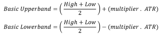
The first thing to do is to average the high and low of the price bar, then we will either add or subtract the average with the selected multiplier multiplied by the ATR as shown in the above formulas.

This will give us two arrays, the basic upper band and the basic lower band which form the first building blocks in the SuperTrend. The next step is to calculate the final upper band and the final lower band using the below formulas.

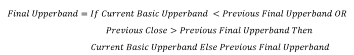
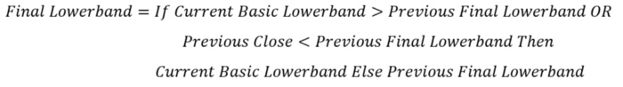
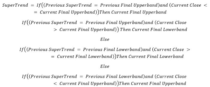
It may seem complicated but most of these conditions are repetitive and in any case, I will provide the Python code below so that you can play with the function and optimize it to your trading preferences. Finally, using the previous two calculations, we can find the SuperTrend.

def supertrend(data, multiplier, high, low, close, atr_col, where):
    
    data = adder(data, 6)
    
    for i in range(len(data)):
        
            data[i, where] = (data[i, high] + data[i, low]) / 2
            
            data[i, where + 1] = data[i, where] + (multiplier * data[i, atr_col])
            
            data[i, where + 2] = data[i, where] - (multiplier * data[i, atr_col])
    
    for i in range(len(data)):
        
        if i == 0:
            
            data[i, where + 3] = 0
            
        else:  
            
            if (data[i, where + 1] < data[i - 1, where + 3]) or (data[i - 1, close] > data[i - 1, where + 3]):
                
                data[i, where + 3] = data[i, where + 1]
            
            else:
                
                data[i, where + 3] = data[i - 1, where + 3]
    
    for i in range(len(data)):
        
        if i == 0:
            
            data[i, where + 4] = 0
            
        else:  
            
            if (data[i, where + 2] > data[i - 1, where + 4]) or (data[i - 1, close] < data[i - 1, where + 4]):
                
                data[i, where + 4] = data[i, where + 2]
            
            else:
                
                data[i, where + 4] = data[i - 1, where + 4]
      
    for i in range(len(data)):
        
        if i == 0:
            
            data[i, where + 5] = 0
        
        elif (data[i - 1, where + 5] == data[i - 1, where + 3]) and (data[i, close] <= data[i, where + 3]):
            
            data[i, where + 5] = data[i, where + 3]
        
        elif (data[i - 1, where + 5] == data[i - 1, where + 3]) and (data[i, close] >  data[i, where + 3]):
            
            data[i, where + 5] = data[i, where + 4]
        
        elif (data[i - 1, where + 5] == data[i - 1, where + 4]) and (data[i, close] >= data[i, where + 4]):
            
            data[i, where + 5] = data[i, where + 4]
        
        elif (data[i - 1, where + 5] == data[i - 1, where + 4]) and (data[i, close] <  data[i, where + 4]):
            
            data[i, where + 5] = data[i, where + 3]   
            
    data = deleter(data, where, 5)

data = jump(data, 1)       
    
    return data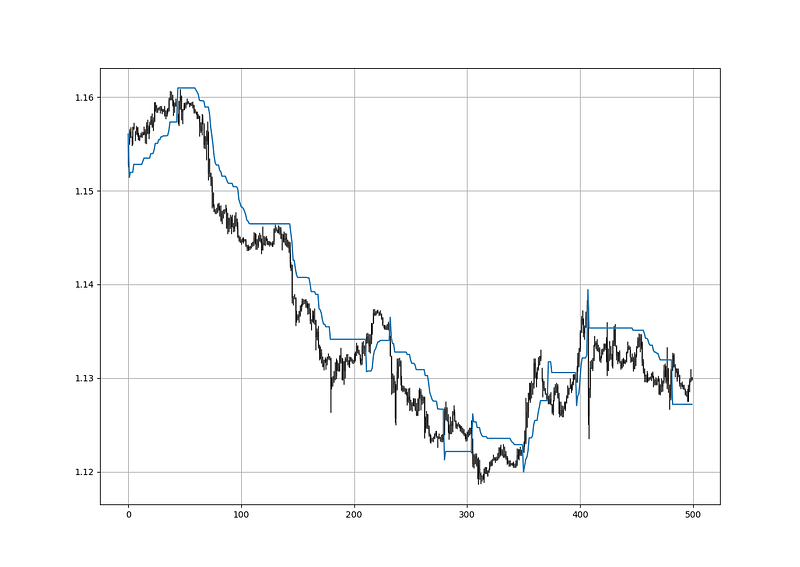

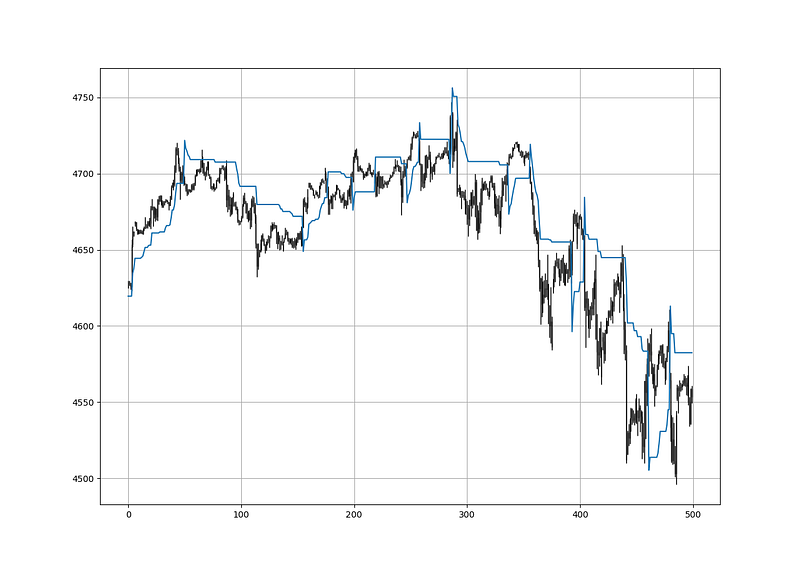
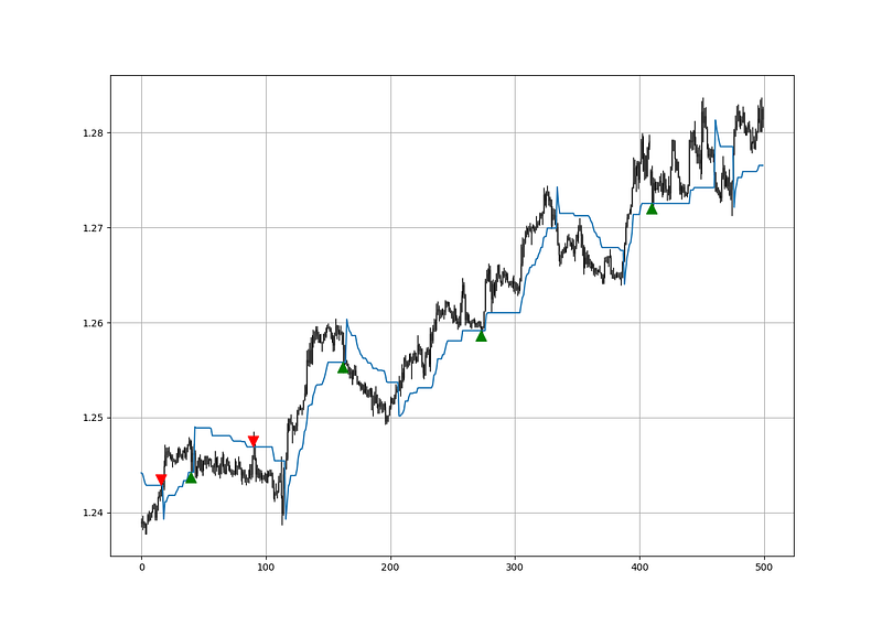
The above chart shows the hourly values of the EURUSD with a 10-period SuperTrend (represented by the ATR period) and a multiplier of 3.00.

The way we should understand the indicator is that when it goes above the market price, we should be looking to short and when it goes below the market price, we should be looking to go long as we anticipate a bullish trend. Remember that the SuperTrend is a trend-following indicator. The aim here is to capture trends at the beginning and to close out when they are over.

Make sure to focus on the concepts and not the code. You can find the codes of most of my strategies in my books. The most important thing is to comprehend the techniques and strategies.

Check out my weekly market sentiment report to understand the current positioning and to estimate the future direction of several major markets through complex and simple models working side by side. Find out more about the report through this link:

Creating the Strategy

A pull-back happens whenever the market surpasses or breaks the SuperTrend line and then comes back to to test it before continuing the initial move. The below are the rules of the strategy:

• A long (Buy) signal is generated whenever the market surpasses the SuperTrend line and comes back to touch it on the condition that the line is flat.
• A short (Sell) signal is generated whenever the market surpasses the SuperTrend line and comes back to touch it on the condition that the line is flat.

The reason we are looking for a flat line is that it signals a ranging condition which improves the possibility of a better reaction.

my_data = atr(my_data, lookback, 1, 2, 3, 4)    
my_data = supertrend(my_data, multiplier, 1, 2, 3, 4, 5)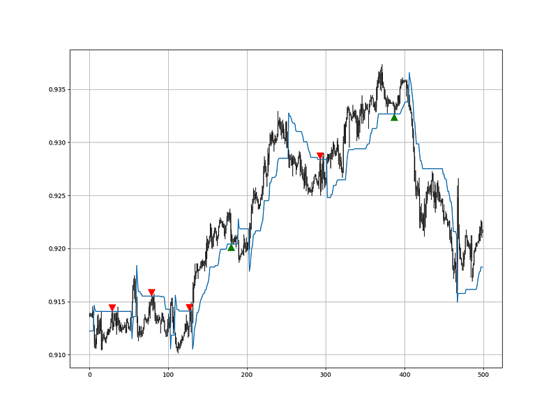

The code to create the pull-back signals can be written as follows:

def signal(data, high_price, low_price, close_price, supertrend_column, buy_column, sell_column):
    
    data = adder(data, 2)
    
    for i in range(len(data)):
        
       if data[i, close_price] > data[i, supertrend_column] and data[i - 1, close_price] < data[i - 1, supertrend_column]:
           
           for a in range(i + 1, len(data)):
               
               if data[a, low_price] <= data[a, supertrend_column] and \
                  data[a, supertrend_column] == data[a - 1, supertrend_column] and \
                  data[a, close_price] > data[a, supertrend_column]:
                   
                   data[a, buy_column] = 1
                   break

elif data[i, close_price] < data[i, supertrend_column] and data[i - 1, close_price] > data[i - 1, supertrend_column]:
           
           for a in range(i + 1, len(data)):
               
               if data[a, high_price] >= data[a, supertrend_column] and \
                  data[a, supertrend_column] == data[a - 1, supertrend_column] and \
                  data[a, close_price] < data[a, supertrend_column]:
                   
                   data[a, sell_column] = -1
                   break           
                   
    return data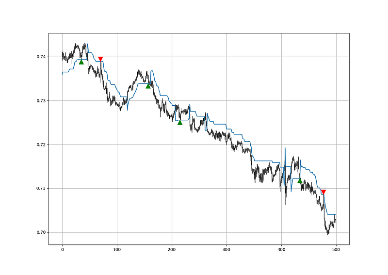

We must combine the strategy with an indicator that confirms the direction, preferably an RSI or a Stochastic oscillator.

Summary

To sum up, what I am trying to do is to simply contribute to the world of objective technical analysis which is promoting more transparent techniques and strategies that need to be back-tested before being implemented.

This way, technical analysis will get rid of the bad reputation of being a subjective and scientifically unfounded.

Medium is a hub to interesting reads. I read a lot of articles before I decided to start writing. Consider joining Medium using my referral link (at NO additional cost to you).

I recommend you always follow the the below steps whenever you come across a trading technique or strategy:

• Have a critical mindset and get rid of any emotions.
• Back-test it using real life simulation and conditions.
• If you find potential, try optimizing it and running a forward test.
• Always include transaction costs and any slippage simulation in your tests.
• Always include risk management and position sizing in your tests.

Finally, even after making sure of the above, stay careful and monitor the strategy because market dynamics may shift and make the strategy unprofitable.