Summary

This context discusses the differences between One Big Table (OBT) and Star Schema in building an analytical data model, highlighting their advantages, disadvantages, and use cases.

Abstract

The context presents two methodologies for building an analytical data model: One Big Table (OBT) and Star Schema. OBT simplifies the database structure by storing all data in a single table, making it easy to manage and query, but it has disadvantages such as redundancy and limited flexibility. Star Schema, on the other hand, is a more complex structure that represents complex relationships between different entities, making it more flexible and efficient for intricate data structures. The context also discusses the use of Domain-Driven Design (DDD) in application development and its impact on data modeling, as well as the use of operational storage for storing dimensions and fact data. The context concludes by discussing the advantages of preserving the star schema and the possibility of using both approaches for specific use cases.

Bullet points

Two methodologies for building an analytical data model are One Big Table (OBT) and Star Schema.
OBT simplifies the database structure by storing all data in a single table, making it easy to manage and query, but it has disadvantages such as redundancy and limited flexibility.
Star Schema is a more complex structure that represents complex relationships between different entities, making it more flexible and efficient for intricate data structures.
Application developers use Domain-Driven Design (DDD) to design their data models, which helps identify core domain entities and map them to dimension table columns and foreign key relationships.
Dimensions are stored in an OLTP database like Postgres, while fact data is stored in an event store like Kafka.
For OBT, the join between the Customer, Movie, and Rental tables must be performed to build the OBT, which can be executed in real-time in a stream processor for fresh data or as a batch process in the OLAP database.
Preserving the star schema has advantages such as complex ETL or ELT not being needed, dimensional tables being easily replicated into the OLAP using change data capture (CDC) and UPSERT, and query flexibility being maximized.
Both approaches can be used for specific use cases, with OBT being used for real-time analytical use cases and a real-time OLAP database supporting UPSERTS for dimensional tables in a star schema.

One Big Table (OBT) vs Star Schema

Two methodologies stand out when building an analytical data model: One Big Table (OBT) and Star Schema. Let’s quickly go over them.

What Is OBT?

“One Big Table” (OBT) is a database design approach in which all the data is stored in a large table. There are no relations between tables in this schema, and all the information is contained within a single structure. This design simplifies the database structure, making it easy to manage and query.

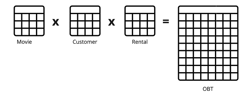
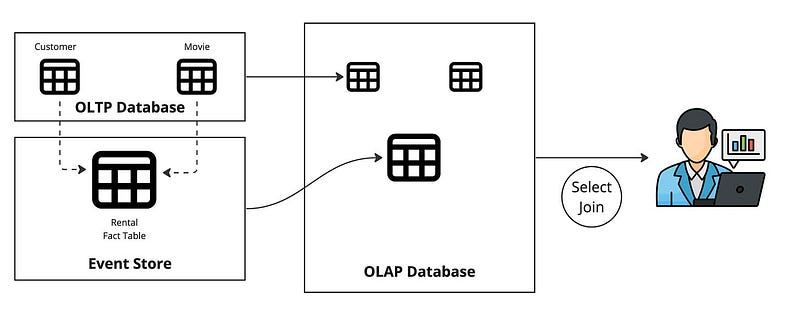
The image above is an example of an OBT that joins Movie, Customer, and Rental tables. This approach can include two or more tables joined together. The OBT table has more rows and columns. This is because all tables’ rows and columns are included in OBT. A downfall of OBT is redundancy since the same information may be repeated across rows, leading to increased storage requirements and potential inconsistency. This creates maintenance challenges where updates, inserts, and deletes can be less efficient and more error-prone in OBT, especially when dealing with changes that affect multiple rows or relationships.

Another disadvantage is OBT’s limited flexibility. OBT might lack the flexibility to represent complex relationships between different entities. This can be a significant drawback when dealing with intricate data structures.

An advantage that OBT has is its simplicity. OBT simplifies database design by consolidating all data into a single table. This simplicity makes understanding, implementing, and managing easier, especially for smaller datasets or less complex applications. Querying can be straightforward with all data in one table, reducing the need for expensive and complex JOIN operations commonly associated with relational databases. For certain use cases, OBT can offer good performance as there are fewer tables and relationships to navigate.

Although, data doesn’t come denormalized from the application domain. So the question begs:

When do we do the JOIN to build One Big Table?

Before we answer that question, let’s first look at how the data may arrive from applications.

Star Schema and Domain Driven Design

Application developers design their data models to represent their domain. Domain-Driven Design (DDD) is an approach to software development that emphasizes a deep understanding of the business domain and incorporates that understanding into the software model. Software models include generated code representing in-memory objects, serialization formats, and persistence definitions like a star schema. DDD is the blueprint for persistent data structure.

DDD helps identify core domain entities, which become dimensions in the Star Schema. Their attributes and relationships map directly to dimension table columns and foreign key relationships.

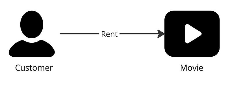
In the diagram below, there are two entities: Customer and Movie. A customer rents a movie, and this defines a relationship.

A customer will have a set of attributes, for example:

Customer ID
First Name
Last Name
Email
Address

Likewise, the movie entity:

Movie ID
Title
Release
Genre

The entities are the dimensions in a star schema. The rent (or Rental) relationship also has attributes such as:

Customer ID
Movie ID
Purchase Date
Expiration Date
Price

The data in the application will tend to be modeled using DDD principles, which keeps the data normalized and aligned with the star schema. This means the data will also be transmitted normalized to any analytical system. But where does the data emit from?

Operational Storage

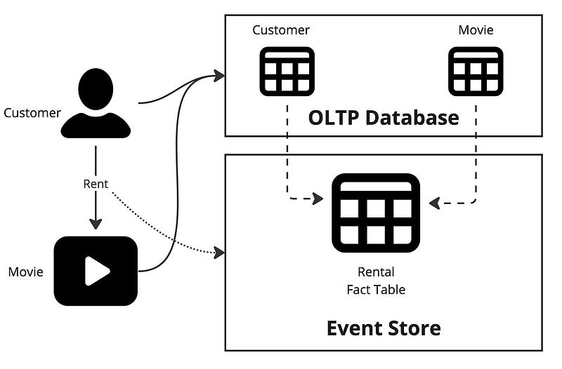
The dimensions are stored in an OLTP database like Postgres on the operational domain where the application lives. The Rental data is stored in an event store like Kafka. Why is this?

Customers and Movies data change slowly. The size of these tables should fit in the OLTP database, but Rentals will not. Rentals tend to be immutable and append-only. If a customer rents a movie, that event is inserted into the Rental table. A new record is appended for every movie rental for every customer. This table will grow very fast. If you choose to put fact data into an OLTP database, you must implement your retention policy by deleting older records.

Where to do the JOIN

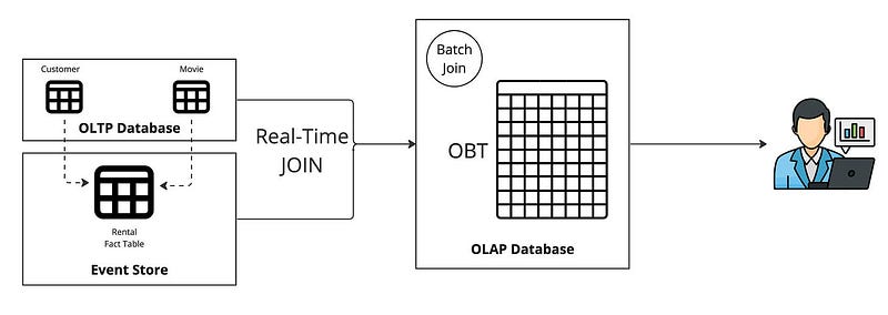
For OBT, you must perform the JOIN between the Customer, Movie, and Rental tables to build the OBT. The join to build the OBT can be executed in real-time in a stream processor for fresh data or as a batch process in the OLAP database. Streaming the data into the OLAP gives you fresh data and does so incrementally. This means instead of processing the entire dataset when batching; the OBT is updated with only the changes.

When choosing the OBT approach, it is important to leverage columnar storage. Any analytical query performed on the OBT will likely not return all columns. Especially as wide as an OBT can get. Read more on columnar storage from Barkha Herman.

Star Schema Alternative

As stated earlier, denormalization for analytical workloads has its advantages. It also has a disadvantage with maintenance challenges: updates, inserts, and deletes can be less efficient and more error-prone in OBT. So, what will it look like if you preserve the star schema?

The advantages of preserving the star schema are:

Complex ETL or ELT is no longer needed.
Dimensional tables can easily be replicated into the OLAP using change data capture (CDC) and UPSERT.
Query flexibility is maximized.

Query flexibility is the ability to execute a query that spans multiple indexes in a data store. It also refers to the ease of querying and manipulating data, such as joining, filtering, aggregating, or sorting.

By leveraging a real-time OLAP database, you can consume data from a streaming platform like Kafka, Redpanda, or Pulsar with the advantage of using columnar storage for analytical workloads.

Why not both?

You can use both approaches by exposing an OBT and a star schema for specific use cases. You must build the OBT from the stream processor for real-time analytical use cases. You’ll need a real-time OLAP database supporting UPSERTS for dimensional tables in a star schema.

To better understand when to use OBT vs star schema, read Chapter 4 in this early-release book Streaming Databases; you will find this diagram below. It will help you understand push/pull queries and materialized views.

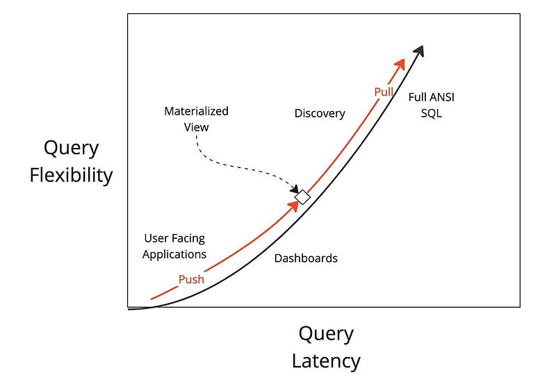
Here is a quote from the book:

If you think about it, the applications that require the lowest latencies would benefit the most from using push queries instead of pull queries. The diagram shows how you can balance between push and pull queries. The box in the middle represents the materialized view. It balances the heavy lifting of push queries with the flexibility of the pull query. How you balance is completely decided by your use case. If the box moves down along the line, the materialized view provides less flexible queries but is more performant. Conversely, as the box moves up, the more flexible the pull queries become but the queries execute at higher latencies. Together, push and pull queries work to find the right balance between latency and flexibility.