
Notes on Gaussian functions, the Gaussian integral, and the Normal Distribution
The Normal distribution is a Gaussian probability distribution. Gaussian probability distributions are functions designed to reflect principles of the central limit theorem which states that a population sample will tend towards the expected value with a sufficiently large random sample and that values farther away from the expected value will occur less frequently. Then there’s the Gaussian integral which is the definite integral of a Gaussian function integrated over the entire real line. These three topics, Gaussian functions, the Gaussian Integral, and Gaussian probability distributions are so inter-woven that I thought it would be best to attempt to address all three of them in one go (I was wrong about that but that’s a topic for a different article). First, we’ll look into what the general definition of a Gaussian function is, then we’ll take a look at the Gaussian integral whose result is necessary in determining the normalization constant for the normal distribution. Lastly, we’ll use the information and understanding we’ve collected and derive the equation for the normal distribution.
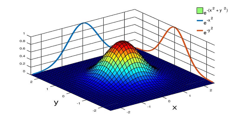
First, lets get a clear understanding of what a Gaussian function actually is. A Gaussian function (or just “Gaussian”) is a function that composes the exponential function exp(x) with a concave quadratic function such as −(ax^2+bx+c) or −(ax^2+bx) or just −ax^2. The result is a family of functions that take on the shape of the infamous “bell curve”.
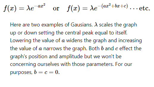

Most people are familiar with these classes of curves because they’re so prolifically used in probability and statistics most notably as the probability density function of a normally distributed random variable. In these cases the function has coefficients and parameters that both scale the amplitude of the “bell”, vary its standard deviation (its width), and translate the mean, all while normalizing the area under the curve (scaling the bell so that the area under the curve always equals 1). The result is a Gaussian function outfitted with what appears to be a host of modifiers to effect these results.
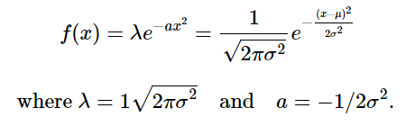
Ok, so you recognize this as the equation of a normal distribution with mean = μ and standard deviation = σ. Comparing it to the general form of a Gaussian λ exp(-ax^2), we can see that:
- The term (x−μ)^2 is just how we employ the mean μ in a way that translates the graph left or right along the x axis, which is all we really want the mean to do. If μ=0 then our graph is centered at 0.
- The variance σ^2, as you know, is a measure of the random variable’s variance — that is, how spread out the data is and its there in both the exponent and the leading coefficient. This is important, because as we narrow or widen the graph using a=1/(2σ^2), we want to simultaneously scale the graph using λ=1/√2πσ^2. In this way, the area under the graph remains 1.
The leading coefficient λ is sometimes expressed as 1/Z where Z=√2πσ^2 and it’s this fact that brings us to one of the main points of the article: √2πσ^2 is sometimes referred to as the normalization constant for a normal distribution of one independent variable at other times its 1/√2πσ2 that’s called the normalizing constant. In either case we have π in the term and we have to ask ourselves where it comes from? Its usually associated with circles, radial symmetry, and/or polar coordinates. So how does a function of a single variable end up with π as one of its normalizing parameters in the leading coefficient?
I can’t tell you why π shows up in the normalizing constant but I can tell you how it’s determined that it needs to be there. The answer lies in the fact that the integral we must take in order to determine a normalizing constant for the normal distribution doesn’t yield to traditional techniques of integration. We have to employ a “trick” that will involve radial symmetry and polar coordinates. If your a fan of Youtube you can find videos explaining the method; a few of which you can find here, here, and here.
The Gaussian Integral
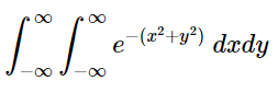
The indefinite integral ∫ exp(x^2) dx is famously impossible to solve in terms of elementary functions. No methods of integration available to us can be used to solve for the anti-derivative. U substitution and integration by parts simply will not work.

The definite integral, however, can be computed. In fact, as we’ll see, and as stated above, we have to first square a Gaussian function resulting in a two variable function in x and y that has a two dimensional graph with radial symmetry. This allows us to convert our rectangular coordinate system into a polar coordinate system where we can take the integral using more familiar techniques of integration (i.e., substitution). Then, we simply take the square root of the result (because we squared the integral in the beginning) and wah-la, we have our answer which, by the way, will be √π. and… who ever said math wasn’t fun!
Squaring the Gaussian integral
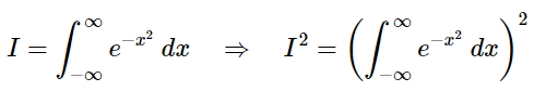
The first step in this method is to square the integral — that is, we convert the one dimensional Gaussian into a two dimensional Gaussian which will allow us to use techniques from multi-variable calculus to solve for the integral.
which can be re-written as:
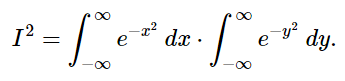
These two integrals, written in x and y, are equivalent; so it’s the same thing as squaring the single integral in x. Also, because both variables x and y are independent, we can move them in and out of the second integral symbol as we choose allowing us to write:
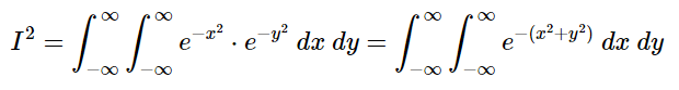
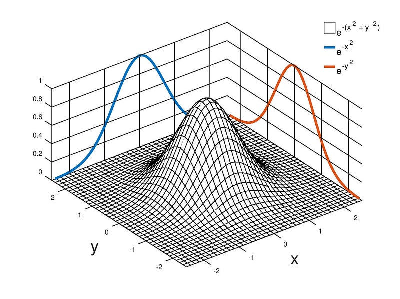
If your unfamiliar with solving double integrals don’t be alarmed. You simply integrate using the inside variable first resulting in a single integral. Then integrate using the variable your left with, the outside variable. But we’re not going to do that just yet. Notice that when we squared the integral we ended up with, in graphical terms, a conically shaped two dimensional, radially symmetric, Gaussian. Writing the integral in terms of x and y leaves us with −(x^2+y^2) as the exponent on e. These two facts give us a clue as to what the next step should be.
Converting to polar coordinates
The tricky part in this solution is that we have to convert our double integral that’s in rectangular coordinates to a double integral in polar coordinates.
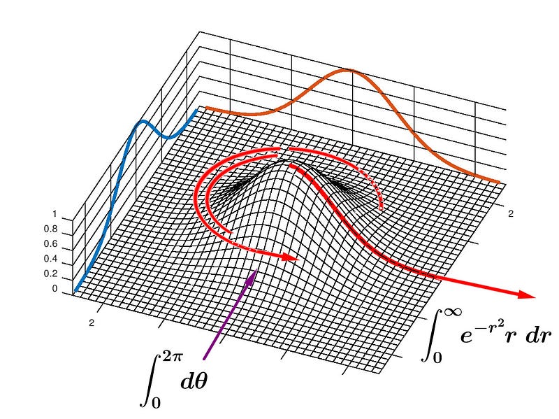
In order to integrate over the entire infinite area in polar coordinates, we first integrate exp(−r²) with respect to the radius r which starts at x=0 and extends to infinity. The result is an infinitely thin wedge that looks like half of our original one dimensional Gaussian curve. Then we rotate the wedge about the origin once, and accumulate an infinite number of these infinitesimally thin wedges. That is — we integrate as θ goes from 0 to 2π.
We currently have a double integral that looks like this:
Thanks to Pythagoras, we can replace −(x^2+y^2) in the exponent with r^2. That’s obvious. But we still have to convert our differentials from rectangular to polar.
As far as converting the differentials goes, let me simply state that:
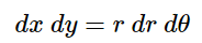
If you’d like a geometrically based argument for why this is so you can find it here or if you prefer a more analytic approach you can find that here. In any case, our double integral now looks like this:
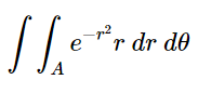
Adding in the appropriate bounds of integration as described above:
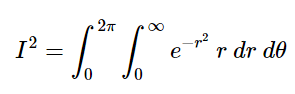
If we set u=r^2 then du=2r and we can write (for the inner integral):
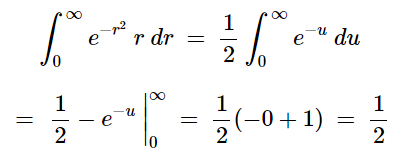
then solving for the outer integral, we have:
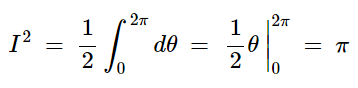
Therefore:

Remember this result. It becomes important when we’re solving for the normalization constant in the next section.
Deriving the normal distribution function
We now have the tools necessary to derive the function for the normal distribution. We’re going to do this in two steps. The first is to determine the probability density function we’re going to need. This means re-casting -a- in terms of λ resulting in a function whose area under the curve is always 1 regardless of the value chosen for λ. Then we’ll re-cast λ in terms of the random variable’s variance σ^2. To do this we’ll integrate the term for variance over the entire real line resulting in the term we’ll need for the normalizing constant in the leading coefficient √2πσ^2, also in the term we’ll need in the denominator of the exponent 2σ^2. We’ll use integration by parts to solve the integral for variance. Most of the instruction for this section I got from this Youtube video posted by Mathoma a little over five years ago.
Derivation of the probability density function
We’re going to start with our generalized Gaussian f(x)=λ exp(−ax^2) and recall that the area under the normal distribution must be equal to 1 so we’ll start by setting the value of our generalized Gaussian, integrated over the entire real line, equal to 1:
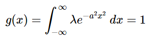
Notice that we’ve modified our Gaussian slightly by replacing -a- with a^2. Why do we want to do this? Because it makes it possible to solve this integral using U-substitution. Why can we do this? Because -a- is an arbitrary constant — therefore, a^2 is also just an arbitrary constant. So, solving using U-substitution, we let u=ax and du=a dx. This means dx=du/a. Further, since λ and 1/a are constants, we can move them outside of the integral symbol yielding:
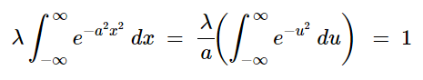
We know from the above discussion on the Gaussian Integral that the value of the integral on the right is equal to √π. This allows us to write:
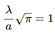
and solving for -a- allows us to write:
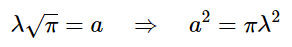
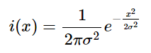
Now that we’ve discovered the relationship between λ and -a-, necessary so that the area under our modified Gaussian is always equal to 1, we can further modify our Gaussian, substituting πλ^2 for a^2 and write:
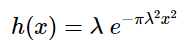
The area under this curve is always 1 regardless of the value of λ. This is our probability density function.
Determining the normalizing constant
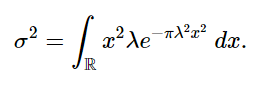
There’s one more thing we have to do before we have our normalized probability distribution function. We have to re-write λ as a function of the random variable’s variance σ^2. As stated above, this is going to involve integrating the expression for variance over the entire real line and we’re going to employ integration by parts to do this.
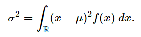
If we’re given a probability density function f(x) and a mean μ, then variance is defined as the deviation from the mean squared (x−μ)^2 times the probability density function f(x) integrated over the entire real line:
We’re going to assume μ=0 and since we already have our probability density function h(x) we can write:
Solving this integral using integration by parts we have:
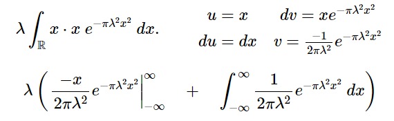
The first term zeros out because the x^2 term in the exponent goes to infinity much faster than the −x term in the numerator of the leading coefficient leaving us with:
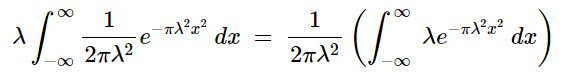
Notice that the integrand on the right is our probability density function which we already know evaluates to 1 when integrated over the entire real line. This results in:
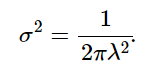
Solving for λ we get:
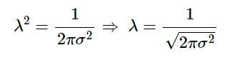
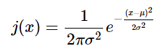
and substituting 1/√2πσ^2 for λ into our modified Gaussian (i.e., our probability density function) we get:
The only thing left to do is put the mean μ into the numerator of the exponent so that we can translate the graph along the x axis depending the the value of μ:
Edit: 02/01/2022: I changed the image and modified the second paragraph in the converting to polar coordinates section in order to correct an error and to better reflect the process discussed.
Thank you so much for reading. If you thought this article was a good read please remember to clap and follow. If you want to make a one time donation to help support my writing projects you can buy me a coffee ☕ or you can become a medium member using this link in which case a portion of your membership fee will go to me. Thank you again for reading this.