#30DaysOfNLP

NLP-Day 7: Topic Modeling With TF-IDF

Implementing a term frequency-inverse document frequency vectorizer from scratch.

Yesterday, we improved our numerical representation of a text by creating a Bag-Of-Words containing the normalized term frequencies. We also vectorized our frequency dictionary, allowing us to perform some more interesting mathematical operations.

However, we still have no way to distinguish between documents across the whole corpus. We have no way of determining the topic by simply relying on the term frequency.

In the following sections, we’re going to tackle that problem.

We will learn about the concept of the term frequency-inverse document frequency (TF-IDF). As complicated as it may sound, it’s not. And to understand things even better, we will compute TF-IDF by hand in a step-by-step fashion.

So take a seat, don’t go anywhere, and make sure to follow #30DaysOfNLP: Topic Modeling With TF-IDF.

Term frequency-inverse document frequency

Up until now, we exclusively relied on the word count or term frequency to determine the importance of certain tokens to a particular document.

This approach, however, is flawed.

In the previous episodes, we saw that the term frequency of common stop words can skew the overall picture quite heavily.

Just because the token "the" appears multiple times in a document doesn’t mean its story is revolving around a commonly used grammatical article in the English language. What kind of story would that be, anyway?

So we need a way to measure the importance of a word to a particular document with respect to the total occurrences across the whole corpus.

Let’s assume we possess a corpus of every book ever written about artificial intelligence. “Artificial intelligence” would almost always appear multiple times in every book or document. But that doesn’t provide any new information to determine the topic or to distinguish the documents.

Something like “Decision Trees”, or “Support Vector Machines” might not occur across the whole corpus. But in the document where it does, we have new information to know what the text might be all about.

TF-IDF provides a “rarity” measure.

The score increases the more frequently a term occurs. However, it decreases the more often the term appears across multiple documents. We can also think of TF-IDF in this way: “How strange is it that this token is in this document?”

TF-IDF is our first step into the realm of topic analysis.

Before implementing an example by hand, we need to know how to calculate TF-IDF.

Pretty straightforward calculations.

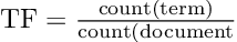
We already know how to compute the term frequency (TF) by simply dividing the word count for a certain term by the total word count of the document.

The inverse document frequency (IDF) can be computed by dividing the total number of documents of a corpus by the number of documents containing our specific term.

Note: We apply a log transformation in order to avoid exponential differences in frequency.

TF-IDF is simply the product of TF and IDF.

TF-IDF from scratch

We know how to calculate TF-IDF, what it means, and why it’s a useful measure.

Now, let’s apply our knowledge and compute the term frequency-inverse document frequency from scratch.

First of all, we import the necessary libraries and create our corpus, containing 4 documents. For demonstrating purposes, we work with a simple nursery rhyme.

Once we created our corpus we’re ready to proceed.

We will use the TreebankWordTokenizer to build our lexicon, containing all unique tokens, except the punctuations.

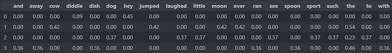
Now, we can compute the normalized term frequency for every token in each document. We store the results in a data frame which makes it easier to visualize the results.

We create an empty data frame with an index for every document and a separate column for each unique token in our lexicon.

Next, we iterate over all documents and create a Bag-Of-Words by utilizing the collections.Counter object. Dividing the word count for a specific term by the number of unique tokens, we obtain the normalized term frequency.

The results, stored in our data frame look like the following.

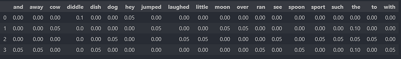
By looking at the results, we can already tell that the term frequency alone doesn’t provide enough information to distinguish or determine the topic.

Thus, we need to compute the inverse document frequency, in order to improve our representation.

We start by creating an empty data frame and obtaining the number of documents in our corpus.

Next, we iterate through each document and term in our lexicon. If the term appears in a document, we store the value 1 in our data frame. By taking the sum for each column over all documents, we obtain the number of documents containing a specific term.

Finally, we calculate the inverse document frequency.

We simply divide the number of documents by the number of documents containing a term. After applying the numpy.log()function we store the values in our data frame.

It’s time for the last step. Tying everything together.

Pretty straightforward.

We basically just multiply both data frames (TF, IDF) and obtain a new one with the term frequency-inverse document frequency. Normalizing the data with sklearn.preprocessing.normalize() creates a unit vector of length 1 for each row.

Note: We apply the normalizing in order to compare our solution later to the sklearn’s implementation.

Now, we can visualize the results.

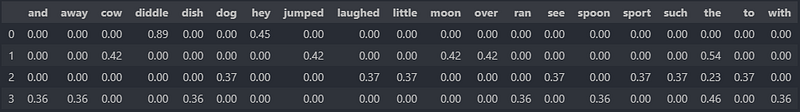
This looks pretty nice.

Just by looking at the TF-IDF scores in the second row, we can tell the document covers something about a “jumping cow”. Sounds reasonable enough.

TF-IDF seems to work very well. However, we had to do a lot of work to get there. Luckily, there exist several tools and libraries to make our lives a lot easier.

Libraries: TfidfVectorizer

In the last section, we computed the TF-IDF scores from scratch.

This was a lot of work. And a lot of code.

Fortunately for us, sklearn comes with an implementation of the TfidfVectorizer which basically does the same job. In a few lines of code.

Let’s take a look and compare the results with our implementation.

And this is it. Much less code. Much faster.

Now, we can visualize the data frame and compare the results.

Looks like we nailed it.

These are the same results as in our implementation from scratch.

Conclusion

In this article, we learned what TF-IDF means, why it’s useful, and even how to compute it from scratch. We also compared our solution to the much easier to use implementation of the sklearn library.

We improved our numerical representation of a given text a lot. However, we still just consider only the number of times a word appears.

In the following episodes, we’re going to take the next step: Entering the world of semantic analysis, providing us with new ways to model the meaning, the topic of a document.

So take a seat, dust off your notebooks, make sure to follow, and never miss a single day of the ongoing series #30DaysOfNLP.

Enjoyed the article? Become a Medium member and continue learning with no limits. I’ll receive a portion of your membership fee if you use the following link, at no extra cost to you.

References / Further Material:

• Hobson Lane, Cole Howard, Hannes Max Hapke. Natural Language Processing in Action. New York: Manning, 2019.