
Neural Networks from Scratch: N-Layers Perceptron — Part 3
Developing deep neural networks from scratch with Mathematics and Python

Unlike traditional machine learning frameworks, deep neural networks are extremely powerful because it can capture highly non-linear relations between the features and target. And the degree of non-linearity is usually controlled by adjusting the depth of the neural network, or the number of Hidden Layers it contains.
But how should deep neural networks be applied? Because the complexity of relations in data set scale with the number of features, deep neural networks are typically ideal for unstructured data or data containing numerous features (n columns). In addition, deep neural networks perform best with sufficient data distribution — less likelihood of over-fitting —with several training examples (m rows).
In the following tutorial, we will explore the workings and issues of building a deep neural network — a true Multi-layer Perceptron — from scratch. Mathematical foundations and notations follow from Part 1 and important ideas such as activation functions, mini-batches and Stochastic Gradient Descent with Momentum are brought forward from Part 2 of the series.
P.S. This series on neural networks is designed to be highly exhaustive, hence if uncertain, please revert to Part 1 and Part 2 to revisit some concepts or mathematical notations.
This article is last part of the 3-part series on Multi-Layer Perceptron of the neural networks:
Part 1: Neural Networks from Scratch: Logistic Regression Part 2: Neural Networks from Scratch: 2-Layers Perceptron Part 3: Neural Networks from Scratch: N-Layers Perceptron
In this article, we will walk through the general architecture of an N-Layer Perceptron, the issues with having several Hidden Layers and how to counter them, and finally code out a deep neural network from scratch, using only Numpy!
P.S. If you are eager to see the codes first, feel free to skip to the end of the article.
Without further delay, let’s get started :)
1. General Architecture of N-Layer Perceptron
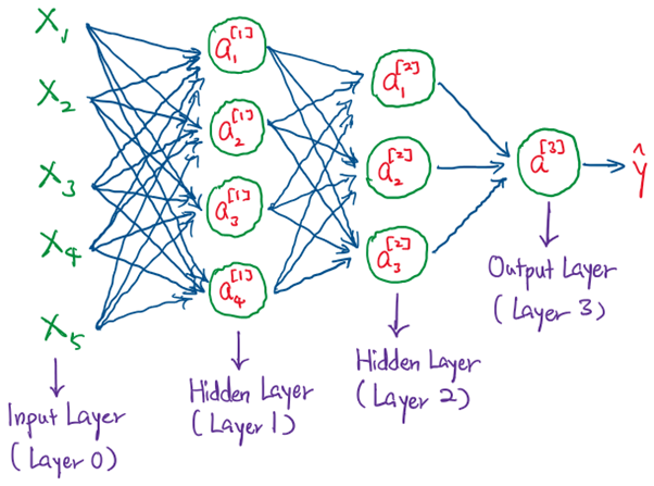
In Part 2, we have seen there is one Hidden Layer in the 2-Layer Perceptron. But for other Multi-Layer Perceptrons, there can be arbitrarily number of Hidden Layers. Hypothetically, we have discussed that these additional Hidden Layers add greater degree of non-linearity into the computation of the output, mainly due to the presence of the activation functions. But semantically, what do these Hidden Layers represent?
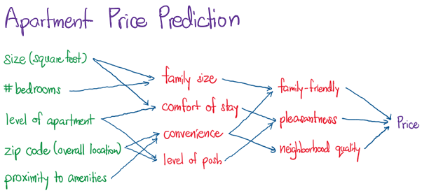
In short, these represent streamlined features that are computed and refined over the process of forward and back propagation. Deep neural networks are essentially learning the best possible feature representations in each Hidden Layer for the data input. By considering only the significant weight components in each layer, we illustrate how a 3-Layer Perceptron (shown above) can explain a regression problem — Apartment Price Prediction.
Some may also ask that instead of making a neural network deep (many Hidden Layers), why not make it wide instead (1 Hidden Layer with many neurons). It turns out that for this shallow neural network to perform as well as a deep neural network, it requires exponentially more neurons as compared to that of the deep neural network, making computation complexity more infeasible.
1.1 Forward and Back Propagation
Now, let us walk through the schema and Mathematics behind Forward and Back Propagation, as illustrated in the sketch below:
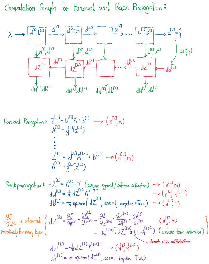
The computation graph for Forward Propagation is very much similar to what we have seen in Part 1 and 2, but for Back Propagation, there is crucial difference. We see that the partial derivative of cost function, J with respective to Z (dZ[L]) is back propagated iteratively at each layer, and is dependent on the previous dZ[L+1], gradient of current activation dA/dZ and previous weights W[L+1]. The value of activation also plays a big part in back propagation since it affects the value of dW, and thus changes W.
From this mathematical perspective, on hindsight, we can understand the need for activation functions, as explained in Part 2, to be more centered about the origin to compute more symmetric gradient values. In addition, we also understand the pros and cons of different activation functions (refer to Part 2) to avoid the issue of Vanishing Gradients and Exploding Gradients.
i.e. Relu activations suffer from Exploding Gradients because activation values are uncapped, and Tanh activations suffer from Vanishing Gradients because dA/dZ are close to zero for huge range of values.
2. Vanishing and Exploding Gradients
As their names explain, Vanishing and Exploding Gradients refer to the partial derivative of cost function, J with respective to Z, or dZ[L], that trends towards zero and infinity respectively as they are back propagated (multiplied) to earlier layers. Hence, the deeper the neural network (greater number of Hidden Layers), the higher the probability of Vanishing/Exploding Gradients happening in earlier layers.
In Exploding Gradients problem, the accumulation of large derivatives backwards results in the model being very unstable in training and achieving wildly fluctuating losses, as large changes in the model weights creates a very unstable network.
On the other hand, in Vanishing Gradients, the accumulation of small gradients results in a model incapable of effective learning since the weights and biases of the initial layers, which tends to learn the core features of the data, become unchanged by small gradients.
Fortunately there are some techniques to overcome these issues, apart from using suitable activation functions. Namely, we will discuss: Weight Initialization
2.1 Weight Initialization
Random weight initialization sometimes pose a problem by generating uneven activation values, depending on the number of neurons in the previous layer. As such, the very first activation values produced may be slightly too large or too small, planting the seed for Vanishing or Exploding Gradients later on in training.
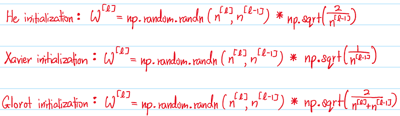
Research has shown that regimes such as He Initialization, Xavier Initialization and Glorot Initialization are effective at initializing weight values that are neither too large or too small across all layers in the neural network. This is because the randomized weight values are somewhat averaged across the number of weights in the Hidden Layer, producing weights that are scaled according to each layer. This results in initial activation values in a comfortable Goldilocks zone.
3. Tendency to Over-fit
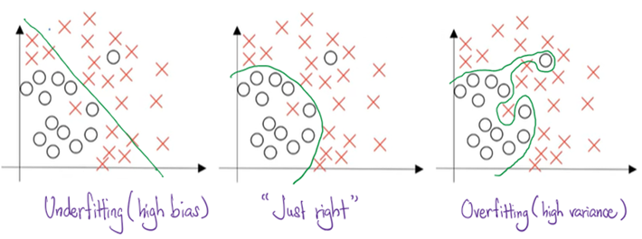
Another thorny issue in training large neural networks is its tendency to over-fit to the training set. What is over-fitting? When the neural network is too large compared to the complexity in the data set, training the model through Gradient Descent would arrive at an optimum that predicts all or almost all data points correctly in the training set. However, when the same model is evaluated on the test set, it performs much worse. What is happening?
Generally the larger the neural network, the better it is at capturing non-linear relation between features and targets at Gradient Descent convergence. When the complexity of the neural network exceeds that of the data set, the model assumes extra patterns in relation between features and targets in order to squeeze all training data into the model fit. This does not bode well with the test set which follows a more general pattern between features and targets.
It is almost impossible to determine the complexity of the data set and engineer a neural network with the optimal depth (number of Hidden Layers) and optimal width (number of neurons). Hence, the way to achieve the best fit for a particular data set is to apply a sufficiently complex neural network with regularization and early stopping.
3.1 Regularization
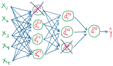
One important technique to lower the complexity of the neural network architecture is to ‘deactivate’ some of the neurons which are less important to lowering the cost function during Gradient Descent, i.e., reducing their weights closer to zero. This process called regularization, reduces prevents these neurons from learning redundant patterns in feature-target relation, while reducing the average of loss function only to a small extent. In particular, we will focus on something called the L2 Regularization, in which we will adjust the cost function, and consequently the gradient descent computation as such:
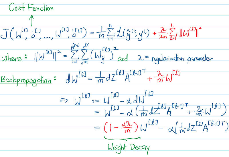
By including weight values into the cost function, the Gradient Descent must account for weights when calculating the cost. And larger weights that insignificantly lower the average of loss functions will be penalized. Following the adjustment of the cost function to include the L2 regularization term (in red), dW and W are similarly adjusted from calculus logic. From the equation above, we also clearly see that the weight values are penalized for every iteration of Gradient Descent, which is why sometimes the L2 regularization is also called Weight Decay.
In addition, in using L2 regularization, the regularization parameter, lambda, must be tweaked, and the value of lambda determines the strength of the regularization.
The beauty of L2 regularization is such that we do not need to determine the complexity of the neural networks by ourselves, but rather through the process of Gradient Descent, the algorithm will automatically decide which neurons to knock out in order to lower complexity to the right fit of the data.
3.2 Early Stopping with Development Set
Yet even with L2 regularization, we do not have an objective measure of when a model is over-fitting or under-fitting. It is hard to obtain a balance, by repeatedly adjusting the regularization parameter and the number of epochs, until we achieve a good result on the test set empirically. And even then, we do not have an impartial estimate of how to model is actually performing, because the end result is biased and tuned towards the test set.
Hence, often in deep learning, we randomly segregate another data set from the training set, called the development set (dev set), whose loss and accuracy can be evaluated along with the training set, at every epoch of training. The result on the development set then gives a statistical estimate whether the model is already over-fitting or under-fitting.
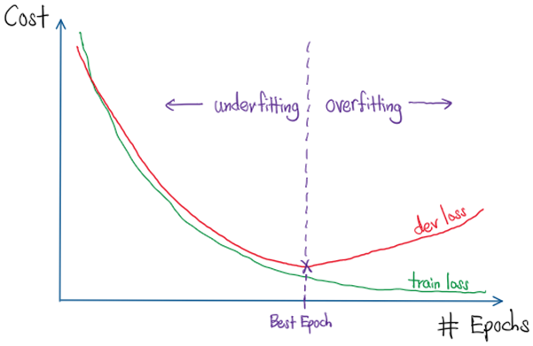
When the learning rate is tuned correctly, the train loss should decrease with every epoch, as the Gradient Descent marches towards to point of convergence. Similarly the dev loss should decrease in tandem. However, at certain point the dev loss would start to increase and deviates from the train loss, and that indicates the onset of over-fitting.
The idea of Early Stopping is to terminate the model training prematurely before the number of epoch expires to retrieve the parameter values (weights and biases) at the end of the best epoch, relative to the dev set. In Early Stopping, we set the Patience parameter which is the number of epochs to train past the best epoch obtained. When the Patience parameter is exceeded without an improvement in dev loss, the training terminates and the best epoch is retrieve. Otherwise, with an improvement in dev loss, the next best epoch is recorded and the Patience ‘timer’ is reset.
Thus, Early Stopping with the dev set achieves a model best-fitted on the dev set. Because the best fit is biased towards the dev set, the model should then be evaluated on the test set to obtained an impartial result.
4. Bonus: Batch Normalization for Deep Networks
So far, we have seen numerous techniques to improve the various aspects of deep neural networks, for instance:
- Improve Optimization and Convergence (Part 2) — Mini-batch Gradient Descent — Gradient Descent with Momentum
- Prevent Vanishing and Exploding Gradients — Use the right activation functions — Apply better weight initialization (He Initialization etc.)
- Reduce Overfitting — Apply L2 Regularization — Early Stopping of training with test set
In this section, we will discuss about another important technique — Batch Normalization — which can improve all these aspects of neural networks simultaneously, enabling us to build very deep networks.
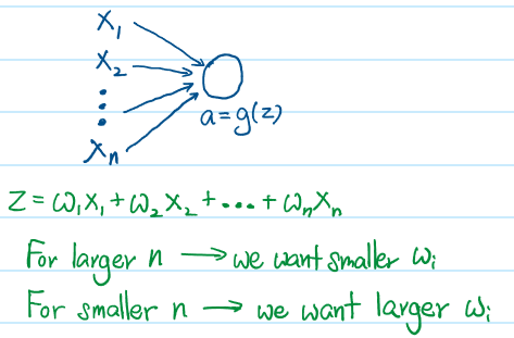
One small but important detail that we have omitted so far is input normalization, which means applying standard normalization to the input vector before feeding it to the neural network, as shown below:
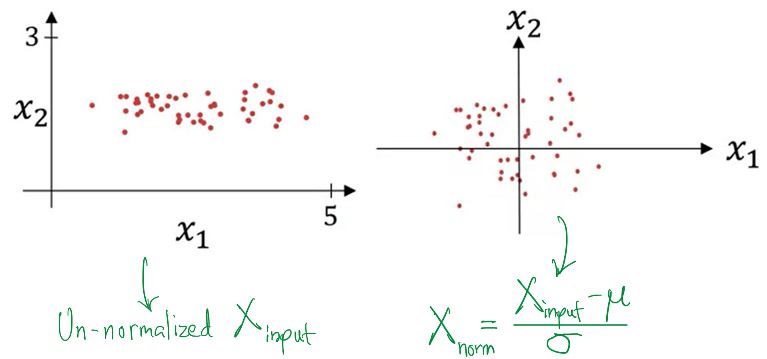
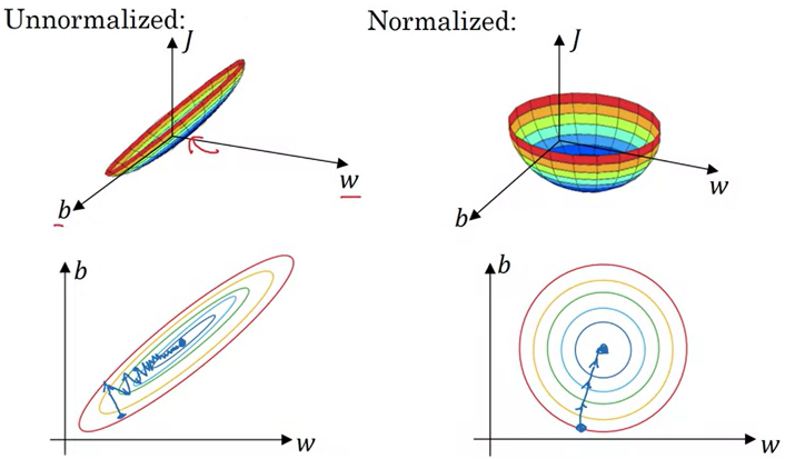
Notice that the standard normalization allows the data to become origin-centered and spread out more evenly around the origin within a small numerical window. In the context of Logistic Regression, this means that the corresponding weights can follow a similar distribution, making Gradient Descent much smoother, more stable and faster, as shown below:
The Batch Normalization follows a similar idea to the input normalization, except that the normalization occurs in the Hidden Layers with respect to each mini-batch, in the context of Mini-Batch Gradient Descent. The idea is that, even when the input vectors are normalized, as Forward Propagation progresses into deeper layers, the Z outputs can have arbitrarily different distribution, or even become very large or very small. Apart from slowing down convergence with uneven Z values, very large or small Z outputs can cause Vanishing and Exploding Gradients. Hence applying Batch Normalization mitigates these issues.
Below we illustrate the process of Batch Normalization in one particular Hidden Layer, with respect to one mini-batch:
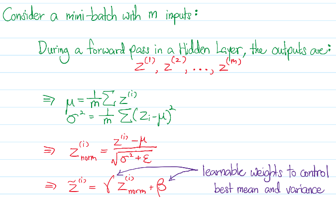
Notice that in our algorithm, Batch Normalization is applied on the Z values, instead of the activations, A. In addition, there are weights γ and β to be learnt during gradient decent to determine the optimal Gaussian distribution for the Z values.
Also note that the mean μ and sigma σ are computed for each mini-batch forward pass. The rolling average of μ and σ are also computed and recorded as parameters when the model finished training, such that they can be applied during testing and inference of unseen data.
Apart from improving convergence and mitigating Vanishing/Exploding Gradients, the Batch Normalization also introduces a slight regularization effect. Since each mini-batch has different distribution statistics, the learnt μ and σ parameters generalizes the input distribution.
Finally, without the Batch Normalization, distributions of activation from each Hidden Layer can shift more wildly with different mini-batches, making learning unstable and optimization difficult. This phenomenon is called Internal Covariate Shift. With Batch Normalization, activations are kept within similar distribution and scale between mini-batches, improving stability of training.
5. The N-Layer Perceptron — Code from Scratch
Finally, we are ready to code the N-Layer neural network from scratch, modeling with an arbitrary number of Hidden Layers, utilizing the concepts mainly from Part 2 and this article, such as the usage of activation functions, mini-batch Gradient Descent with Momentum, L2 regularization, Early Stopping with Development Set and more!
Note: We exclude applying the Batch Normalization in the network model, nonetheless baking this feature into the neural network should not be too difficult. We leave this to the reader as an exercise of creativity.
We will then proceed to evaluate the model on the MNIST data set (60,000 training examples) provided by Tensorflow, and compare its performance against the Tensorflow’s Keras API. The MNIST data set are image data of numerical characters 0 to 9 in grayscale format and the task is to predict the characters from their images.
Note that the pixel values of the image data are integers 0 to 255, where the larger the values indicate brighter pixels. In an important preprocessing step, we have to normalize their image data by dividing the pixel values by 255. Large feature values from the Input Layer can delay convergence, and worse, increase tendency for Exploding Gradients as they lead to large activation values initially.
Without further delay and explanation, I will leave to the grandeur and results of the N-Layer neural network from scratch!
6. Final Thoughts
What a breathtaking ride! I hope you have enjoyed this series on Neural Network from Scratch, as much as I had in creating them for you. I apologize if the writing style has been overly technical, but please take great care in going through the concepts in these 3 articles, as they are extremely informative and cover the intricacies of Neural Network a great deal. Below are the links to the previous articles:
Finally tell me about your thoughts about neural networks, and leave some comments on what you like to see in the future. I look forward to creating more technical algorithms from scratch, and hope for your support!
P.S. The codes in this article can be found in my GitHub
Cheers! _/\_
Thanks for reading! If you have enjoyed the content, pop by my other articles on Medium and follow me on LinkedIn.
Support me! — If you are not subscribed to Medium, and like my content, do consider supporting me by joining Medium via my referral link.


