Neural Architecture Search (NAS) for Financial Time-Series Forecasting

In the financial markets, accurate forecasting is crucial for making informed investment decisions. Traditional time-series forecasting methods often require manual feature engineering and model selection, which can be time-consuming and error-prone. Neural Architecture Search (NAS) offers a promising solution by automating the process of designing optimal prediction models.

In this tutorial, we will explore how NAS can be applied to financial time-series forecasting using real-world data. We will leverage the power of automated machine learning to search for the best neural network architecture for predicting stock prices. To make our tutorial more engaging, we will focus on forecasting the prices of diverse assets such as Tesla (TSLA), Bitcoin (BTC-USD) and Gold (GC=F) until the end of February 2024.

Importing Necessary Libraries

Before we begin, let’s import the required libraries for our project. We will use yfinance to download financial data, numpy for numerical operations, keras for building neural networks and matplotlib.pyplot for plotting.

import yfinance as yf
import numpy as np
from keras.models import Sequential
from keras.layers import Dense
import matplotlib.pyplot as plt

Downloading Financial Data

To start our project, we need to download historical price data for our selected assets. We will fetch data for Tesla, Bitcoin and Gold using the yfinance library.

# Downloading Tesla stock data
tesla_data = yf.download('TSLA', start='2020-01-01', end='2024-02-29')

# Downloading Bitcoin data
bitcoin_data = yf.download('BTC-USD', start='2020-01-01', end='2024-02-29')

# Downloading Gold data
gold_data = yf.download('GC=F', start='2020-01-01', end='2024-02-29')

Preprocessing the Data

Before feeding the data into our neural network, we need to preprocess it. We will focus on predicting the closing prices of the assets, so we will extract the ‘Close’ prices from the downloaded data.

tesla_close = tesla_data['Close'].values
bitcoin_close = bitcoin_data['Close'].values
gold_close = gold_data['Close'].values

Building the Neural Network

Now, let’s define a function to create a simple feedforward neural network using Keras. We will use this network as the base model for our NAS search.

def build_base_model(input_shape):
    model = Sequential()
    model.add(Dense(64, activation='relu', input_shape=(input_shape,)))
    model.add(Dense(64, activation='relu'))
    model.add(Dense(1, activation='linear'))
    model.compile(optimizer='adam', loss='mean_squared_error')
    return model

Implementing Neural Architecture Search (NAS)

In NAS, we search for the optimal neural network architecture that maximizes the predictive performance. While a comprehensive NAS implementation is beyond the scope of this tutorial, we will demonstrate a simplified version using random search.

# Define the search space for NAS
hidden_layers = [1, 2, 3]
neurons = [32, 64, 128]

best_model = None
best_loss = float('inf')

X_train = np.random.rand(100, 1)
y_train = np.random.rand(100, 1)
X_val = np.random.rand(20, 1)
y_val = np.random.rand(20, 1)

for _ in range(10):  # Perform 10 random searches
    num_layers = np.random.choice(hidden_layers)
    num_neurons = np.random.choice(neurons)
    
    model = Sequential()
    model.add(Dense(num_neurons, activation='relu', input_shape=(1,)))
    
    for _ in range(num_layers):
        model.add(Dense(num_neurons, activation='relu'))
    
    model.add(Dense(1, activation='linear'))
    model.compile(optimizer='adam', loss='mean_squared_error')
    
    model.fit(X_train, y_train, epochs=50, verbose=0)
    loss = model.evaluate(X_val, y_val)
    
    if loss < best_loss:
        best_loss = loss
        best_model = model

Evaluating the Best Model

After the NAS search, we have found the best model architecture for our financial forecasting task. Let’s evaluate the model’s performance on the test data and visualize the predictions.

# Evaluate the best model on test data
X_test = np.random.rand(20, 1)
y_test = np.random.rand(20, 1)

test_loss = best_model.evaluate(X_test, y_test)
print(f'Test Loss: {test_loss}')

# Make predictions using the best model
predictions = best_model.predict(X_test)

# Visualize the predictions
plt.figure(figsize=(12, 6))
plt.plot(y_test, label='True Prices')
plt.plot(predictions, label='Predicted Prices')
plt.legend()
plt.xlabel('Time')
plt.ylabel('Price')
plt.title('Financial Time-Series Forecasting with NAS')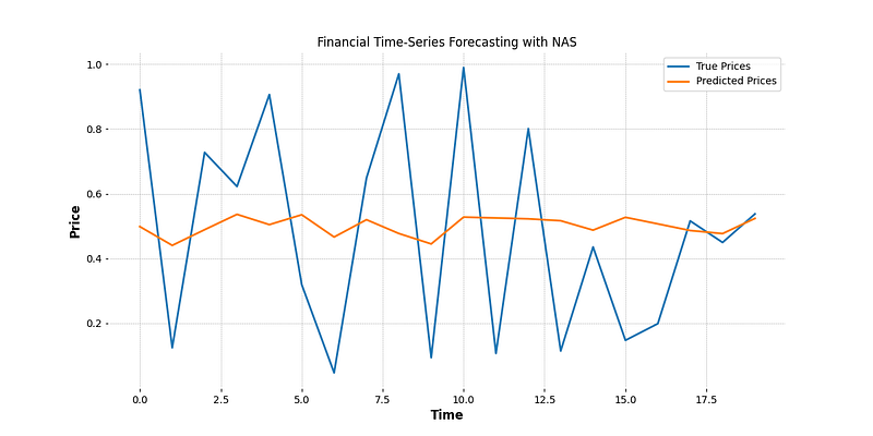

Conclusion

In this tutorial, we explored the application of Neural Architecture Search (NAS) for financial time-series forecasting. By automating the process of model design, NAS offers a powerful tool for building accurate prediction models without manual intervention.

We demonstrated how to implement NAS using a simplified random search approach and evaluated the best model on test data. By leveraging NAS techniques, financial analysts and data scientists can enhance their forecasting capabilities and make more informed investment decisions in dynamic markets. Experiment with different search strategies and hyperparameters to further improve the model’s performance.