Random Forest Classifier in Python

End-to-end note to handle both categorical and numeric variables at once

Content

Data Preprocessing (a trick to handle categorical features and NAs automatically)
Train the RF classifier
Evaluate the classifier (accuracy, recall, precision, ROC AUC, confusion matrix, plotting)
Feature Importance
Tune the hyper-parameters with Random Search

Now let’s get started, folks!

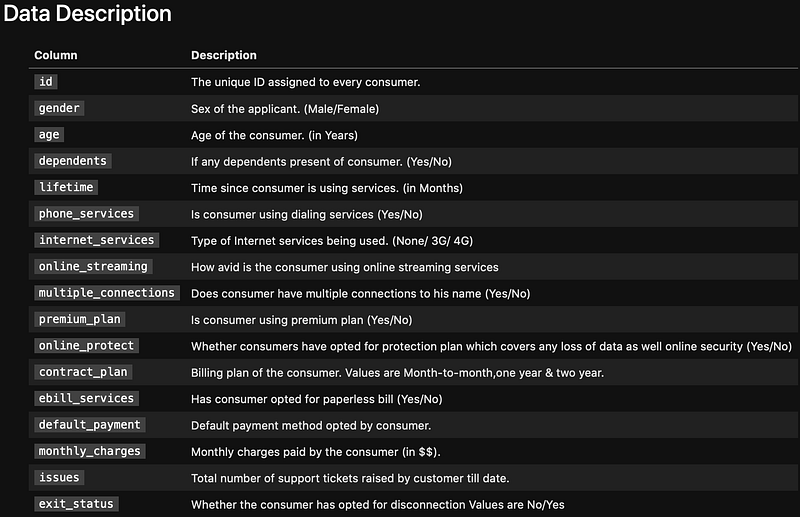
Data Description

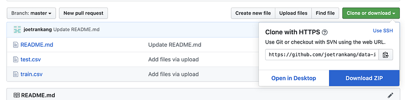
In this article, I am using the dataset taken from my real technical test with a tech company for a data science position. You can get the data here (click Download ZIP).

Disclaimer: all the information described in the data are not real.

The exit_status here is the response variable. Note that we are only given train.csv and test.csv. Thetest.csvdoes not have exit_status, i.e. it is only for prediction. Hence the approach is that we need to split the train.csv into the training and validating set to train the model. Then use the model to predict theexit_status in the test.csv.

This is a typical Data Science technical test where you are given around 30 minutes to produce a detailed jupyter notebook and result.

1. Data Preprocessing

import pandas as pd
import numpy as np
import matplotlib.pyplot as plt

data = pd.read_csv('train.csv')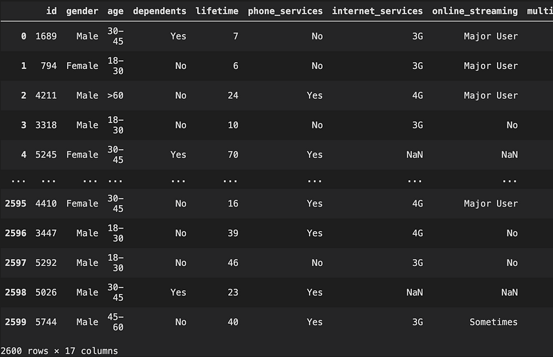

Oops, we saw NaN, let’s check how many NaN we have

Check NAs

data.isnull().sum()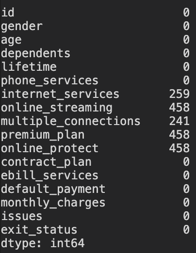

Since there are 2600 rows in total, the number of rows with NAs here is relatively small. However, I do not remove NAs here because what if the test.csv dataset also has NAs, then removing the NAs in the train data will not enable us to predict the customers' behaviour where there are NAs. However, if the test.csv does not have any NAs, then we can go ahead and remove the NAs in the train dataset. But let’s first check out the test.csv

test = pd.read_csv('test.csv')
test.isnull().sum()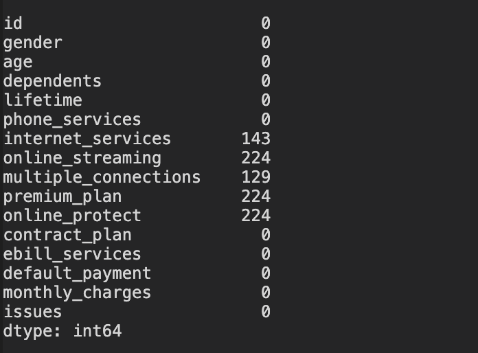

As expected, there are NAs in test.csv. Hence, we will treat NAs as a category and assume it contributes to the response variable exit_status.

Replace Yes-No in exit_status to 1–0

exit_status_map = {'Yes': 1, 'No': 0}
data['exit_status'] = data['exit_status'].map(exit_status_map)

This step is useful later because the response variable must be an numeric array to input into RF classifier. Like I mentioned earlier, RF model is unable to read strings or any non-numeric datatypes.

Split the data into X and y

y = data.pop('exit_status')
X = data.drop('id',axis = 1)

The id column does not add any meaning to our work because it will not affect whether the customer chose to stay or exit, so we should just remove it.

Create training and validating set

seed = 50  # so that the result is reproducible
from sklearn.model_selection import train_test_split

X_train, X_test, y_train, y_test = train_test_split(X,y,test_size=0.333, random_state = seed)

Now, it is time to make NA a category. In Python, NaN is considered NAs. When encoded, those NaN will be ignored. Hence, it is useful to replace NaN with na, which is now a category called ‘na’. This will be taken into account when encoding later on.

X_train = X_train.fillna('na')
X_test = X_test.fillna('na')

Create list of categorical variables to encode

X_train.dtypes

Notice that only categorical variables has dtype = object

Now, let’s create a list of categorical variables

features_to_encode = list(X_train.select_dtypes(include = ['object']).columns)

# Or alternatively,

features_to_encode = X_train.columns[X_train.dtypes==object].tolist()

Create a constructor to handle categorical features for us

This is my favorite step because by recreating this new constructor, I do not need to do any transformation for any X dataframe when passing into the model. This constructor will automatically handle the categorical variables and leave numeric variables untouched. How convenient!!!

from sklearn.preprocessing import OneHotEncoder
from sklearn.compose import make_column_transformer

col_trans = make_column_transformer(
                        (OneHotEncoder(),features_to_encode),
                        remainder = "passthrough"
                        )

The remainder = 'passthrough' allows the constructor to ignore those variables that are not included in features_to_encode.

Now our inputs are ready. Let’s train the RF classifier.

2. Train the RF classifier

Let’s first create our first model. Of course one can start with rf_classifier = RandomForestClassifier(). However, most of the time this base model will not perform really well (from my experience at least, yours might differ). So I always start with the following set of parameters as my first model.

from sklearn.ensemble import RandomForestClassifier

rf_classifier = RandomForestClassifier(
                      min_samples_leaf=50,
                      n_estimators=150,
                      bootstrap=True,
                      oob_score=True,
                      n_jobs=-1,
                      random_state=seed,
                      max_features='auto')

I would recommend to always start with the model where oob_score = True because it is better to use out-of-bag samples to estimate the generalization accuracy. An oob error estimate is almost identical to that obtained by k-fold cross-validation. Unlike many other nonlinear estimators, random forests can be fit in one sequence, with cross-validation being performed along the way.

Now, let’s combine our classifier and the constructor that we created earlier, by using Pipeline

from sklearn.pipeline import make_pipeline
pipe = make_pipeline(col_trans, rf_classifier)
pipe.fit(X_train, y_train)

pipe is a new black box created with 2 components: 1. A constructor to handle inputs with categorical variables and transform into a correct type, and 2. A classifier that receives those newly transformed inputs from the constructor.

y_pred = pipe.predict(X_test)

3. Evaluate the classifier

from sklearn.metrics import accuracy_score, confusion_matrix, precision_score, recall_score, roc_auc_score, roc_curve, f1_score

Accuracy = (TP + TN) / (TP+TN+FP+FN)

Recall = TP / (TP + FN)

Precision = TP / (TP + FP)

F1-score = 2 * Precision * Recall / (Precision+Recall)

In this example, 1 is Positive and 0 is Negative

I will not go through the meaning of each term above because this article is not meant to be a detailed document of Random Forest algorithms. I assume we all know what these terms mean. Of course, if you are unsure, feel free to ask me in the comment section.

Accuracy (fraction of correctly classified samples)

accuracy_score(y_test, y_pred)

print(f"The accuracy of the model is {round(accuracy_score(y_test,y_pred),3)*100} %")

The accuracy of the model is 91.1%

Make probability predictions

train_probs = pipe.predict_proba(X_train)[:,1] 
probs = pipe.predict_proba(X_test)[:, 1]

train_predictions = pipe.predict(X_train)

predict_proba(dataframe)[:,1] gives the predicted probability distribution of class label 1 from the dataframe. This is important to calculate ROC_AUC score. You may ask why class label 1 and not 0. Here is what I got from sklearn document:

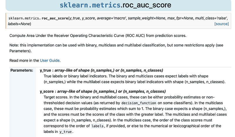
For y_score, ‘The binary case … the scores must be the scores of the class with the greater label’. That is why we need to get label 1 instead of label 0.

print(f'Train ROC AUC Score: {roc_auc_score(y_train, train_probs)}')

print(f'Test ROC AUC  Score: {roc_auc_score(y_test, probs)}')

Train ROC AUC Score: 0.9678578659647703 
Test ROC AUC Score: 0.967591183178179

Now, we need to plot the ROC curve

def evaluate_model(y_pred, probs,train_predictions, train_probs):

    baseline = {}

    baseline['recall']=recall_score(y_test,

                    [1 for _ in range(len(y_test))])

    baseline['precision'] = precision_score(y_test,

                    [1 for _ in range(len(y_test))])

    baseline['roc'] = 0.5

    results = {}

    results['recall'] = recall_score(y_test, y_pred)

    results['precision'] = precision_score(y_test, y_pred)

    results['roc'] = roc_auc_score(y_test, probs)

    train_results = {}

    train_results['recall'] = recall_score(y_train,       train_predictions)

    train_results['precision'] = precision_score(y_train, train_predictions)

    train_results['roc'] = roc_auc_score(y_train, train_probs)

    for metric in ['recall', 'precision', 'roc']:

          print(f'{metric.capitalize()} 
                 Baseline: {round(baseline[metric], 2)} 
                 Test: {round(results[metric], 2)} 
                 Train: {round(train_results[metric], 2)}')

     # Calculate false positive rates and true positive rates

    base_fpr, base_tpr, _ = roc_curve(y_test, [1 for _ in range(len(y_test))])

    model_fpr, model_tpr, _ = roc_curve(y_test, probs)

    plt.figure(figsize = (8, 6))
    plt.rcParams['font.size'] = 16

    # Plot both curves

    plt.plot(base_fpr, base_tpr, 'b', label = 'baseline')
    plt.plot(model_fpr, model_tpr, 'r', label = 'model')
    plt.legend();

    plt.xlabel('False Positive Rate');
    plt.ylabel('True Positive Rate'); plt.title('ROC Curves');
    plt.show();

evaluate_model(y_pred,probs,train_predictions,train_probs)

Recall Baseline: 1.0 Test: 0.92 Train: 0.93 
Precision Baseline: 0.48 Test: 0.9 Train: 0.91 
Roc Baseline: 0.5 Test: 0.97 Train: 0.97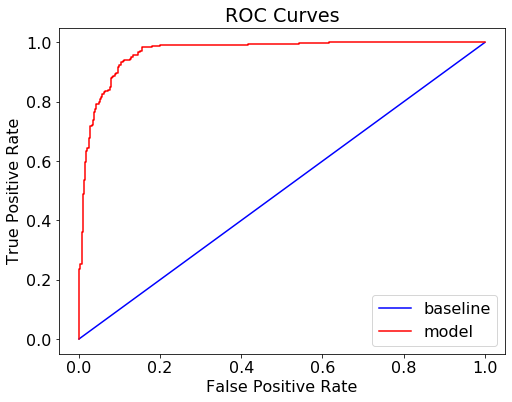

The result looks good. There is very little difference between Test and Train result, indicating that our model does not overfit the data.

Confusion matrix

One can just simply type confusion_matrix(y_test, y_pred) to get the confusion matrix. However, let’s take a more advanced approach. Here, I create a function to plot confusion matrix, which prints and plots the confusion matrix. (Adapted from Source of the code)

import itertools

def plot_confusion_matrix(cm, classes, normalize = False,
                          title='Confusion matrix',
                          cmap=plt.cm.Greens): # can change color

    plt.figure(figsize = (10, 10))
    plt.imshow(cm, interpolation='nearest', cmap=cmap)
    plt.title(title, size = 24)
    plt.colorbar(aspect=4)

    tick_marks = np.arange(len(classes))
    plt.xticks(tick_marks, classes, rotation=45, size = 14)
    plt.yticks(tick_marks, classes, size = 14)

    fmt = '.2f' if normalize else 'd'
    thresh = cm.max() / 2.

    # Label the plot

    for i, j in itertools.product(range(cm.shape[0]),   range(cm.shape[1])):

    plt.text(j, i, format(cm[i, j], fmt), 
             fontsize = 20,
             horizontalalignment="center",
             color="white" if cm[i, j] > thresh else "black")

    plt.grid(None)
    plt.tight_layout()
    plt.ylabel('True label', size = 18)
    plt.xlabel('Predicted label', size = 18)

# Let's plot it out

cm = confusion_matrix(y_test, y_pred)
plot_confusion_matrix(cm, classes = ['0 - Stay', '1 - Exit'],
                      title = 'Exit_status Confusion Matrix')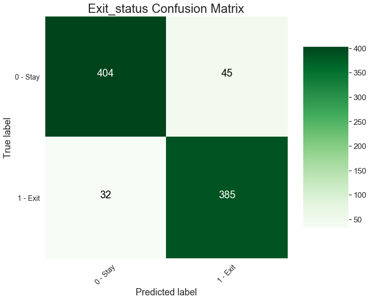

4. Feature Importance

First, let’s inspect how many feature importance values are there in the model

print(rf_classifier.feature_importances_)

print(f" There are {len(rf_classifier.feature_importances_)} features in total")

[7.41626071e-04 6.12165359e-04 1.42322746e-03 6.93254520e-03  2.93650843e-04 1.96706074e-04 1.85830433e-03 2.67517842e-03  1.02110066e-05 2.99006245e-05 6.15325794e-03 1.66647237e-02  4.49100748e-03 3.37963818e-05 1.87449830e-03 1.00225588e-03  3.72119245e-04 1.39558189e-02 8.28073088e-04 3.41692010e-04  1.71733193e-04 7.60943914e-02 1.09485070e-02 1.78380970e-02  1.63392715e-02 2.93397339e-03 1.46445733e-02 1.34849432e-01  1.33144331e-02 4.42753783e-02 3.13204793e-03 4.97894324e-03  6.17692498e-03 2.70959923e-02 1.61849449e-03 7.57024010e-02  2.31468190e-02 4.66247828e-01]

There are 38 features in total

There are 38 features in total. However, there are only 15 columns in X_train. This is because the model pipe automatically encodes the categorical variables in X_train. For example, the gender column in X_train is transformed into 2 columns Female and Male.

Therefore, to match the features to their feature importance values derived from rf_classifier, we need to get all those corresponding columns in the encoded X_train.

Question:

We only have an array of feature importances, but there are both categorical and numerical features, how do we know which value belongs to which feature?

Remember the col_trans, the constructor we created earlier? The col_trans.fit_transform(X_train) will give the encoded X_train.

# Let's look at the first row
print(col_trans.fit_transform(X_train)[0,:])

[ 0.    1.    0.    0.    0.    1.    1.    0.    0.    1.    1.    0.   0.    0.    1.    0.    0.    0.    1.    0.    0.    1.    0.    0.   1.    0.    0.    1.    0.    0.    0.    1.    0.    1.    0.   30.  74.75 14.  ]

# And the first row of X_train
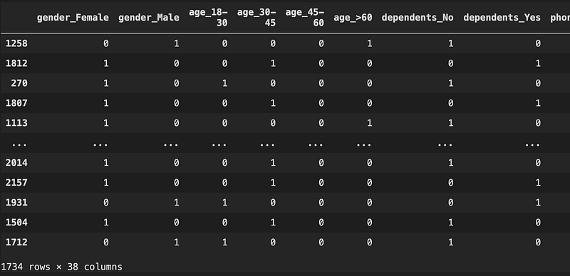
X_train.iloc[0,:]

gender                             Male
age                                 >60
dependents                           No
lifetime                             30
phone_services                      Yes
internet_services                    3G
online_streaming             Major User
multiple_connections                 No
premium_plan                         No
online_protect                       No
contract_plan            Month-to-month
ebill_services                      Yes
default_payment         Online Transfer
monthly_charges                   74.75
issues                               14
Name: 1258, dtype: object

For X_train, there are 3 numeric variables, with values being 30, 70.75 and 14 respectively. For the encoded X_train, these 3 numeric values are placed after all the categorical variables. This means that for the rf_classifier.feature_importances_ all the encoded categorical variables are shown first, followed by the numeric variables

Ok, now that we know, let’s create a proper encoded X_train.

def encode_and_bind(original_dataframe, features_to_encode):

    dummies = pd.get_dummies(original_dataframe[features_to_encode])
    res = pd.concat([dummies, original_dataframe], axis=1)
    res = res.drop(features_to_encode, axis=1)
    return(res)

X_train_encoded = encode_and_bind(X_train, features_to_encode)

The function encode_and_bind encodes the categorical variables and then combine them with the original dataframe.

Cool, now we have 38 columns, which is exactly the same as the 38 features shown in the rf_classifier.feature_importances_ earlier.

feature_importances = list(zip(X_train_encoded, rf_classifier.feature_importances_))

# Then sort the feature importances by most important first
feature_importances_ranked = sorted(feature_importances, key = lambda x: x[1], reverse = True)

# Print out the feature and importances
[print('Feature: {:35} Importance: {}'.format(*pair)) for pair in feature_importances_ranked];

Some features and their importance scores (descending order)

# Plot the top 25 feature importance

feature_names_25 = [i[0] for i in feature_importances_ranked[:25]]
y_ticks = np.arange(0, len(feature_names_25))
x_axis = [i[1] for i in feature_importances_ranked[:25]]

plt.figure(figsize = (10, 14))
plt.barh(feature_names_25, x_axis)   #horizontal barplot
plt.title('Random Forest Feature Importance (Top 25)',
          fontdict= {'fontname':'Comic Sans MS','fontsize' : 20})

plt.xlabel('Features',fontdict= {'fontsize' : 16})
plt.show()

5. Tune the hyperparameters with RandomSearchCV

Since the model performs very well, with high accuracy, precision and recall, there is actually little need to tune the model. However, if our first model did not perform well, the steps below can be taken to tune the model.

Let’s look at the parameters used currently

from pprint import pprint

print('Parameters currently in use:\n')
pprint(rf_classifier.get_params())

Now, I create a grid of parameters for the model to randomly pick and train, hence the name Random Search.

from sklearn.model_selection import RandomizedSearchCV

n_estimators = [int(x) for x in np.linspace(start = 100, stop = 700, num = 50)]

max_features = ['auto', 'log2']  # Number of features to consider at every split

max_depth = [int(x) for x in np.linspace(10, 110, num = 11)]   # Maximum number of levels in tree

max_depth.append(None)

min_samples_split = [2, 5, 10]  # Minimum number of samples required to split a node

min_samples_leaf = [1, 4, 10]    # Minimum number of samples required at each leaf node

bootstrap = [True, False]       # Method of selecting samples for training each tree

random_grid = {'n_estimators': n_estimators,

               'max_features': max_features,

               'max_depth': max_depth,

               'min_samples_split': min_samples_split,

               'min_samples_leaf': min_samples_leaf,

               'max_leaf_nodes': [None] + list(np.linspace(10, 50, 500).astype(int)),

               'bootstrap': bootstrap}

Now, I first create a base model, then use random grid to select the best model, based on the ROC_AUC score, hence scoring = 'roc_auc'.

# Create base model to tune

rf = RandomForestClassifier(oob_score=True)

# Create random search model and fit the data

rf_random = RandomizedSearchCV(

                        estimator = rf,

                        param_distributions = random_grid,

                        n_iter = 100, cv = 3,

                        verbose=2, random_state=seed,

                        scoring='roc_auc')

rf_random.fit(X_train_encoded, y_train)

rf_random.best_params_

rf_random.best_params_

{'n_estimators': 206,
 'min_samples_split': 5,
 'min_samples_leaf': 10,
 'max_leaf_nodes': 44,
 'max_features': 'auto',
 'max_depth': 90,
 'bootstrap': True}

We will do 100 iterations with 3-fold cross validation. More information about the arguments can be found here.

Alternatively, we can use pipe again, so that we don’t need to encode the data

rf = RandomForestClassifier(oob_score=True, n_jobs=-1)

rf_random = RandomizedSearchCV(

                estimator = rf,

                param_distributions = random_grid,

                n_iter = 50, cv = 3,

                verbose=1, random_state=seed,

                scoring='roc_auc')

pipe_random = make_pipeline(col_trans, rf_random)

pipe_random.fit(X_train, y_train)

rf_random.best_params_

Note that the 2 methods might give slightly diffferent answers. This is due to the randomness in selecting the parameters.

# To look at nodes and depths of trees use on average

n_nodes = []

max_depths = []

for ind_tree in best_model.estimators_:

       n_nodes.append(ind_tree.tree_.node_count)

       max_depths.append(ind_tree.tree_.max_depth)

print(f'Average number of nodes {int(np.mean(n_nodes))}')   print(f'Average maximum depth {int(np.mean(max_depths))}')

Average number of nodes 82 
Average maximum depth 9

Evaluate the best model

# Use the best model after tuning

best_model = rf_random.best_estimator_

pipe_best_model = make_pipeline(col_trans, best_model)

pipe_best_model.fit(X_train, y_train)

y_pred_best_model = pipe_best_model.predict(X_test)

The same codes used in Section 3 can be applied here again for ROC and Confusion matrix.

train_rf_predictions = pipe_best_model.predict(X_train)

train_rf_probs = pipe_best_model.predict_proba(X_train)[:, 1]

rf_probs = pipe_best_model.predict_proba(X_test)[:, 1]

# Plot ROC curve and check scores

evaluate_model(y_pred_best_model, rf_probs, train_rf_predictions, train_rf_probs)

Recall Baseline: 1.0 Test: 0.94 Train: 0.95 
Precision Baseline: 0.48 Test: 0.9 Train: 0.91 
Roc Baseline: 0.5 Test: 0.97 Train: 0.98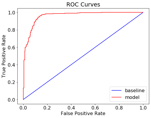

This set of parameters make the model perform just slightly better than our original model. The difference is not huge. This is understandable because our original model already performed well with higher scores (accuracy, precision, recall). So tuning some hyperparameters might not add any significant improvement to the model.

# Plot Confusion matrix

plot_confusion_matrix(confusion_matrix(y_test, y_pred_best_model), classes = ['0 - Stay', '1 - Exit'],

title = 'Exit_status Confusion Matrix')

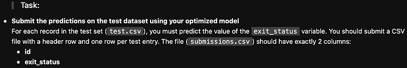
Use the best model on test.csv data

Now that we have the best model, let’s use it for predictions and compile our final answer to submit.

test = pd.read_csv('test.csv')
test_withoutID = test.copy().drop('id', axis = 1)
test_withoutID = test_withoutID.fillna('na')

final_y = pipe_best_model.predict(test_withoutID)
#pipe model only takes in dataframe without ID column.

final_report = test
final_report['exit_status'] = final_y
final_report = final_report.loc[:,['id','exit_status']]

# Replace 1-0 with Yes-No to make it interpretable

final_report= final_report.replace(1, 'Yes')
final_report= final_report.replace(0, 'No')

We see all No. Let’s check to make sure there are Yes in the column too.

final_report.exit_status.value_counts()

No     701
Yes    638
Name: exit_status, dtype: int64

Okay, we are safe~

Save and submit the file

final_report.to_csv('submissions.csv', index=False)

Conclusion

I hope this can be a helpful reference guide for you guys as well. You can use this guide to prepare for probably some technical tests or use it as a cheatsheet to brush up on how to implement Random Forest Classifier in Python. I will definitely keep on updating this as I find more useful functions or tricks that I think can help everyone tackle many data science problems fast, without much need to look up on platforms like StackOverflow, especially when sitting for a technical test, where time is limited.

If there are any other tricks or functions that you think are important, please let me know in the comment section below. Also, I welcome any constructive feedback from everyone.

Thank you for your read. Have a great day and happy programming!