
My Approach To Use the MACD Indicator in the Market — Part 2
A different approach using the same MACD indicator
Here we are again! Welcome to Part 2 about my approach to trading with the MACD indicator. In Part 1, we set the foundation, introducing the core components of the strategy, and explaining how it works. As promised, we’re now going into the specifics, introducing the Percentage Price Oscillator (PPO) and exploring the concept of Expected Value.
But before we proceed, let’s briefly recap the essentials from Part 1.
Main Idea
As you may know, my approach involves using the MACD indicator, but in its percentage version (PPO or Percentage Price Oscillator). To make this approach more understandable, let’s break it down into four crucial components:
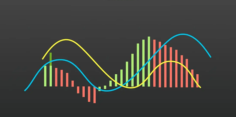
Minimum Distance to Buy: Think of this as your “buying threshold.” It represents the minimum value you want to see in the histogram before you consider buying an asset. In simpler terms, it’s like saying, “I won’t buy unless this is over this value.”
Trend to Buy: This component helps you decide when to buy based on recent changes in the histogram. It’s like looking at recent history to see if the histogram has been going up, or down. Depending on the trend, you may decide to make a purchase or wait.
Maximum Distance to Sell: Just as you have a minimum for buying, you also have a maximum threshold for selling. This means you won’t sell your asset if the histogram is over a certain level.
Trend to Sell: Similar to the Trend to Buy, this helps you decide when to sell based on recent changes in the histogram. It’s about gauging whether the histogram is going up, or down before you make your selling decision.
With all the parameters defined, we’ll look at a certain number of past values when considering these factors. Imagine this like looking back in time to see how the histogram has behaved before making your move. The number of past values you examine is an essential part of your strategy.
Finding the Best Values for Success
Now, let’s move on to the exciting part — how to optimize our approach for maximum success. To do this, we’ll introduce the Percentage Price Oscillator (PPO), which is a variation of the MACD designed to provide a normalized view of market movements.
What is the Percentage Price Oscillator (PPO)?
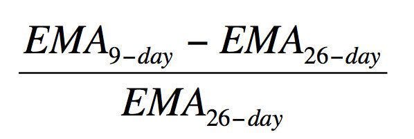
The Percentage Price Oscillator, or PPO, is a modified version of the MACD indicator, tailor-made for traders who want to work with percentages rather than raw price values. Instead of tracking the difference between two Exponential Moving Averages (EMAs) like the MACD, the PPO calculates the percentage difference between these EMAs. This can offer a clearer picture of price trends and make it easier to compare assets with varying price levels.
Before continuing with the rest of the information, if you enjoy reading my articles, please consider hitting the follow button — Diego Degese
Understanding Expected Value (EV)
Before we proceed to optimize our strategy using the PPO, it’s crucial to understand the concept of Expected Value (EV).
Basically, the Expected Value is a generalization of the weighted average. (This definition was taken from wikipedia.com)
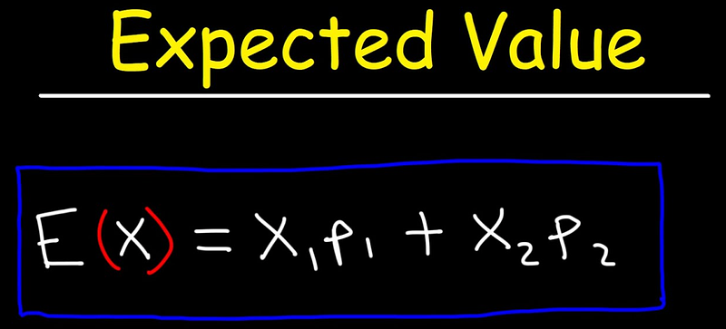
Wow, what are you talking about? Let’s add an example for better understanding. Expected Value, in our case, is calculated by considering two key factors:
- Win Rate (Probability of Success): This represents the likelihood of a trade resulting in a positive return, or in simpler terms, making a profit.
- Positive and Negative P&L (Profit and Loss): These are the financial gains and losses associated with a trade, respectively.
With these components, we can calculate the Expected Value using the following formula:
Expected Value = (Win Rate * Positive P&L) + (1 — Win Rate) * Negative P&L
In simpler terms, it’s a way of quantifying the average profitability of our trading strategy. If the Expected Value is positive, it suggests that, on average, our strategy is expected to yield profits. On the other way, if it’s negative, it indicates an expected average loss.
Well, enough theory for today, let's go and explore the code, but please don’t forget to hit the follow button for more articles like this— Diego Degese.
Source code to optimize the Expected Value using the PPO Histogram
Let’s break down the code step by step to understand its functionality. We will use a genetic algorithm to optimize the trading parameters based on a PPO and the Expected Value.
Import the Required Libraries
import numpy as np
import pandas as pd
import pandas_ta as ta
import pygad
from tqdm import tqdm
Here, we import necessary libraries for data manipulation, technical analysis (pandas_ta), genetic algorithm optimization (pygad), and a progress bar (tqdm).
Define the Constants
# Constants
DEBUG = 0
CASH = 10_000

SOLUTIONS = 30
GENERATIONS = 50

FILE_TRAIN = '../data/spy.train.csv.gz'
FILE_TEST = '../data/spy.test.csv.gz'

TREND_LEN = 7
MIN_TRADES_PER_DAY = 1
MAX_TRADES_PER_DAY = 10
These are constants used throughout the code, such as debugging options, initial cash amount, file paths for training and testing data, genetic algorithm parameters, and trading constraints.
Configure Numpy and Pandas
# Configuration
np.set_printoptions(suppress=True)
pd.options.mode.chained_assignment = None
These lines configure the display options for NumPy and Pandas to make the output more readable and suppress scientific notation.
Load and Preprocess Data
# Loading data, and split into train and test datasets

def get_data():

    train = pd.read_csv(FILE_TRAIN, compression='gzip')
    train['date'] = pd.to_datetime(train['date'])
    train.ta.ppo(close=train['close'], append=True)
    train = train.dropna().reset_index(drop=True)

    test = pd.read_csv(FILE_TEST, compression='gzip')
    test['date'] = pd.to_datetime(test['date'])
    test.ta.ppo(close=test['close'], append=True)
    test = test.dropna().reset_index(drop=True)

    train = train[train['date'] > (test['date'].max() - pd.Timedelta(365 * 10, 'D'))]

    return train, test
This function get_data() loads and preprocesses training and testing data. It includes reading data from CSV files, converting dates, resampling time intervals, and calculating the PPO indicator.
Define the Fitness Function
# Define fitness function to be used by the PyGAD instance
def fitness_func(self, solution, sol_idx):

    # Get Reward from train data
    reward, wins, losses, pnl = get_result(train, train_dates,
                                 solution[           :TREND_LEN*1],
                                 solution[TREND_LEN*1:TREND_LEN*2],
                                 solution[TREND_LEN*2:TREND_LEN*3],
                                 solution[TREND_LEN*3:TREND_LEN*4])

    if DEBUG:
        print(f'\n{reward:10.2f}, {pnl:10.2f}, {wins:6.0f}, {losses:6.0f}, {solution[TREND_LEN*1:TREND_LEN*2]}, {solution[TREND_LEN*3:TREND_LEN*4]}', end='')

    # Return the solution reward
    return reward
This function fitness_func() is used by the genetic algorithm to evaluate the fitness of a solution. It calculates a reward and other trading metrics based on the solution parameters, and the reward is used as the fitness value.
Define a Result Calculation Function
# Define a reward function
def get_result(df, business_dates, min_dist_buy, trend_buy, max_dist_sell, trend_sell, is_test=False):

    # Min/Max Trades
    min_trades = len(business_dates) * MIN_TRADES_PER_DAY
    max_trades = len(business_dates) * MAX_TRADES_PER_DAY

    # Buy & Sell Signals
    buy_mask = True
    sell_mask = True

    for i in range(0, len(min_dist_buy)):

        buy_mask = buy_mask & (df['PPOh_12_26_9'] > min_dist_buy[i])
        sell_mask = sell_mask & (df['PPOh_12_26_9'] < max_dist_sell[i])

        if i == 0: continue

        if trend_buy[i] > 0:
            buy_mask = buy_mask & (df['PPOh_12_26_9'].shift(i - 1) > df['PPOh_12_26_9'].shift(i))
        elif trend_buy[i] < 0:
            buy_mask = buy_mask & (df['PPOh_12_26_9'].shift(i - 1) < df['PPOh_12_26_9'].shift(i))

        if trend_sell[i] > 0:
            sell_mask = sell_mask & (df['PPOh_12_26_9'].shift(i - 1) > df['PPOh_12_26_9'].shift(i))
        elif trend_sell[i] < 0:
            sell_mask = sell_mask & (df['PPOh_12_26_9'].shift(i - 1) < df['PPOh_12_26_9'].shift(i))

    if buy_mask.sum() == 0: # Return if there are no buy signals
        return max(-999999, -len(df) + buy_mask.sum()), 0, 0, 0

    if sell_mask.sum() == 0: # Return if there are no sell signals
        return max(-999999, -len(df) + sell_mask.sum()), 0, 0, 0

    df['signal'] = np.where(buy_mask, 1, 0)
    df['signal'] = np.where(sell_mask, -1, df['signal'])

    # Remove all rows without operations, rows with the same consecutive operation, first row selling, and last row buying
    ops = df[df['signal'] != 0]
    ops = ops[ops['signal'] != ops['signal'].shift()]
    if (len(ops) > 0) and (ops.iat[0, -1] == -1): ops = ops.iloc[1:]
    if (len(ops) > 0) and (ops.iat[-1, -1] == 1): ops = ops.iloc[:-1]

    if len(ops) == 0: # Return if there are no operations
        return -min_trades, 0, 0, 0

    # Calculate the reward / operation
    ops['pnl'] = np.where(ops['signal'] == -1, (ops['close'] - ops['close'].shift()) * (CASH // ops['close'].shift()), 0)

    # Generate the ops
    pnl = ops['pnl'].sum()
    wins = len(ops[ops['pnl'] > 0])
    losses = len(ops[ops['pnl'] < 0])

    # Calculate Expected Value
    valid_ops = ops[ops['pnl'] != 0]
    if len(valid_ops) == 0: # Return if there are no valid operations
        return -min_trades, 0, 0, 0

    if not is_test and (len(valid_ops) < min_trades):
        ev = -min_trades + len(valid_ops) # Penalize if there are less trades than the minimum allowed
    elif not is_test and (len(valid_ops) > max_trades):
        ev = -min_trades # Penalize if there are more trades than the maximum allowed
    else:
        win_rate = wins / (wins + losses) if (wins + losses) > 0 else 0
        ev = win_rate * ops[ops['pnl'] > 0]['pnl'].sum() - (1 - win_rate) * -ops[ops['pnl'] < 0]['pnl'].sum()

    return ev, wins, losses, pnl
This function get_result() calculates trading metrics, including Expected Value (EV), based on input data and trading parameters. It considers aspects like buy and sell signals, trade counts, and profit or loss.
After defining the main functions and constants, we will start using them to do our tests.
Load Train and Test Data
# Get Train and Test data
train, test = get_data()
This line calls the get_data() function to load and preprocess training and testing data.
Calculate Business Days for Train and Test Data
# Calculate Business days for train and test datasets
train_dates = train[['date']].set_index('date').resample('1D').max()
train_dates = train_dates[train_dates.index.dayofweek < 5]

test_dates = test[['date']].set_index('date').resample('1D').max()
test_dates = test_dates[test_dates.index.dayofweek < 5]
These lines calculate business days for both the training and testing datasets, filtering out weekends.
Process Data and Run Genetic Algorithm
# Process data
print("".center(60, "*"))
print(f' PROCESSING DATA '.center(60, '*'))
print("".center(60, "*"))

with tqdm(total=GENERATIONS) as pbar:

    # Define Gene space based on configuration
    gene_space = []

    for i in range(TREND_LEN):
        gene_space.append({'low': -1, 'high': 1.1, 'step': 0.1})

    for i in range(TREND_LEN):
        gene_space.append({'low': -1, 'high': 2, 'step': 1})

    for i in range(TREND_LEN):
        gene_space.append({'low': -1, 'high': 1.1, 'step': 0.1})

    for i in range(TREND_LEN):
        gene_space.append({'low': -1, 'high': 2, 'step': 1})

    # Create Genetic Algorithm
    ga_instance = pygad.GA(num_generations=GENERATIONS,
                           num_parents_mating=5,
                           fitness_func=fitness_func,
                           sol_per_pop=SOLUTIONS,
                           num_genes=len(gene_space),
                           gene_space=gene_space,
                           parent_selection_type="sss",
                           crossover_type="single_point",
                           mutation_type="random",
                           mutation_by_replacement=True,
                           mutation_num_genes=2,
                           keep_parents=-1,
                           random_seed=42,
                           on_generation=lambda _: pbar.update(1),
                           )

    # Run the Genetic Algorithm
    ga_instance.run()
This section of the code sets up the genetic algorithm using PyGAD. It defines the gene space and other GA parameters, runs the GA, and finds the best solution.
Obtain the Best Solution
solution, _, _ = ga_instance.best_solution()
In this line, ga_instance.best_solution() is used to obtain the best solution found by the genetic algorithm. The solution variable will contain the optimized trading parameters that maximize the defined fitness function.
Calculate and Display Training Results
reward, wins, losses, profit = get_result(train, train_dates,
                                          solution[           :TREND_LEN*1],
                                          solution[TREND_LEN*1:TREND_LEN*2],
                                          solution[TREND_LEN*2:TREND_LEN*3],
                                          solution[TREND_LEN*3:TREND_LEN*4],
                                          True)
This section calculates and retrieves various trading metrics for the training dataset using the get_result() function. It uses the best solution's parameters to assess the trading strategy's performance on historical data. The metrics include reward (a measure of the strategy's success), wins (number of winning trades), losses (number of losing trades), and profit (total profit or loss).
Display Training Results
print(f' Best Solution Parameters '.center(60, '*'))
print(f"Min Dist Buy    : {solution[           :TREND_LEN*1]}")
print(f"Trend Buy       : {solution[TREND_LEN*1:TREND_LEN*2]}")
print(f"Max Dist Sell   : {solution[TREND_LEN*2:TREND_LEN*3]}")
print(f"Trend Sell      : {solution[TREND_LEN*3:TREND_LEN*4]}")

print(f' Result (TRAIN) '.center(60, '*'))
print(f"* Reward         : {reward:.2f}")
print(f"* Profit / Loss  : {profit:.2f}")
print(f"* Wins / Losses  : {wins} / {losses}")
print(f"* Win Rate       : {(100 * (wins/(wins + losses)) if wins + losses > 0 else 0):.2f}%")
In this section, the code displays the details of the best solution parameters, including the minimum distance to buy, trend to buy, maximum distance to sell, and trend to sell. These parameters are crucial for understanding the trading strategy.
It also prints the trading results for the training dataset, including the reward, profit or loss, wins, losses, and the win rate. These metrics provide insights into how well the strategy performed on historical data.
Calculate and Display Testing Results
reward, wins, losses, profit = get_result(test, test_dates,
                                          solution[           :TREND_LEN*1],
                                          solution[TREND_LEN*1:TREND_LEN*2],
                                          solution[TREND_LEN*2:TREND_LEN*3],
                                          solution[TREND_LEN*3:TREND_LEN*4],
                                          True)
Similar to the training dataset, this section calculates and retrieves various trading metrics for the testing dataset. It uses the same best solution parameters to assess how the trading strategy would have performed on unseen data.
Display Testing Results
print(f' Result (TEST) '.center(60, '*'))
print(f"* Reward         : {reward:.2f}")
print(f"* Profit / Loss  : {profit:.2f}")
print(f"* Wins / Losses  : {wins} / {losses}")
print(f"* Win Rate       : {(100 * (wins/(wins + losses)) if wins + losses > 0 else 0):.2f}%")
This section prints the testing results, including the reward, profit or loss, wins, losses, and the win rate for the testing dataset. It provides insights into how well the strategy might perform on new data, helping to assess its robustness.
Overall, this part of the code summarizes the key information about the optimized trading strategy, displays the best solution’s parameters, and presents the trading results for both the training and testing datasets, giving you a clear view of the strategy’s performance.
The results with the default parameters
***************** Best Solution Parameters *****************
Min Dist Buy    : [-0.2 -0.9 -0.2 -0.8 -0.5 -1.  -0.7]
Trend Buy       : [ 0. -1.  1.  0.  0.  0.  0.]
Max Dist Sell   : [0.5 0.4 1.  0.8 0.7 0.6 0.9]
Trend Sell      : [-1.  1.  1.  0. -1.  1.  1.]
********************** Result (TRAIN) **********************
* Reward         : 26064.74
* Profit / Loss  : 10242.80
* Wins / Losses  : 11569 / 8668
* Win Rate       : 57.17%
********************** Result (TEST) ***********************
* Reward         : 6176.72
* Profit / Loss  : 735.61
* Wins / Losses  : 2142 / 1635
* Win Rate       : 56.71%
The optimized trading strategy, based on the default parameters, yields promising results. The best solution parameters include minimum distance to buy, trend to buy, maximum distance to sell, and trend to sell values that have been fine-tuned by the genetic algorithm.
In the training dataset, this strategy achieved a profit of $10,242.80. It demonstrated a win rate of 57.17%, indicating a consistent success rate in trading decisions. These results suggest that the strategy has the potential to be highly profitable in a historical context. Furthermore, when tested on unseen data (the testing dataset), it maintained its robustness, delivering a profit of $735.61. The win rate remained strong at 56.71%, reinforcing the strategy’s effectiveness in capturing profitable trading opportunities in different market conditions.
Conclusion
In conclusion, the results obtained from the optimized trading strategy, as showcased through the best solution parameters and performance metrics, are quite promising. These findings open up a lot of possibilities for further research and exploration. It’s worth noting that the strategy’s success is not limited to the specific parameters, timeframes, or datasets used in this analysis. Instead, it underscores the potential for extensive research and experimentation, allowing traders and researchers to fine-tune and adapt the strategy to other market conditions, assets, and timeframes. By going deeper into the strategy’s underlying principles and continuously refining its parameters, there still is some room for finding new insights and enhancing its profitability.
I’ll be waiting for your comments and tests…
If you enjoy my work, please support me on Medium by becoming a member through my referral link, and consider giving it a clap as a small gesture of motivation. Thank you!
Download the full source code, the colab notebook of this article from here.
Twitter / X: https://x.com/diegodegese LinkedIn: https://www.linkedin.com/in/ddegese Github: https://github.com/crapher
Disclaimer: Investing in the stock market involves risk and may not be suitable for all investors. The information provided in this article is for educational purposes only and should not be construed as investment advice or a recommendation to buy or sell any particular security. Always do your own research and consult with a licensed financial advisor before making any investment decisions. Past performance is not indicative of future results.
Did you see my previous articles? Check some of them for more information…
Subscribe to DDIntel Here.
DDIntel captures the more notable pieces from our main site and our popular DDI Medium publication. Check us out for more insightful work from our community.
Register on AItoolverse (alpha) to get 50 DDINs
Join our network here: https://datadriveninvestor.com/collaborate
DDI Official Telegram Channel: https://t.me/+tafUp6ecEys4YjQ1


