Monte Carlo Simulation Theory and Applications in Python

The Monte Carlo Simulation is a numerical analysis technique aimed at estimating the possible outcomes of a certain random event. It is a very powerful method of evaluating integrals where there are no known solutions.

The main idea behind this simulation is that the results are computed based on repeated random sampling and statistical analysis. The technique relies on random sampling, the Law of Large Numbers and the Central Limit Theorem.

1. Monte Carlo Approximation

Suppose we wanted to evaluate the integral:

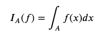
over the domain set 𝐴

We can do so using two different points of view.

a. Using Expectation

We can express this integral as:

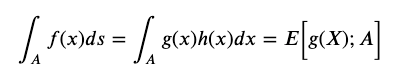
Where,

• 𝑋 is a random variable with a probability density function given by ℎ(𝑥)
• 𝐸[𝑔(𝑋);𝐴] represents the expected value of 𝑔(𝑥) over the set 𝐴

This means we can re-express the integral as an expectation of a function of a random variable over a given set

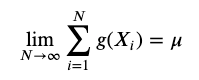
Suppose we have i.i.d. random variables 𝑋1,𝑋2,… with:

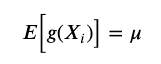
meaning the expectation is equal to the mean

Then, as the number of random variables we simulate increases towards infinity, the sample mean converges to the expected value of the function of the random variables:

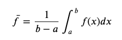
b. Using a Simple Average

We can take the mean of a function with one variable to understand how to apply the Monte Carlo numerical method to solve for the integral of the function.

Let A be the domain (𝑎,𝑏)

By rearranging the distance of the domain 𝑏−𝑎 to the left-hand side we get:

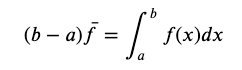
If we were to represent the different outcomes of this function on a uniformly distributed grid and we take the limit as the distribution goes to zero then we would get as a result the solution to this integral.

However, this is extremely computationally expensive, especially when dealing with multiple dimensions.

Approximating the integral:

By expanding the left-hand side and expressing the mean of 𝑓 as the definition of the average, we get a solution that approximates the actual solution of the integral.

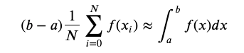
We can approximate the integral by making the 𝑥𝑖 values be a random 𝑥 value on the interval (𝑎,𝑏) and if we take the limit that the number of these 𝑥 values goes to infinity, we will get the value of the integral

2. Simple Integration using the Mean of a Function

We can use Monte Carlo Integration to see how close to this value we can approximate.

We need to:

1. Get the function to integrate
2. The limits of integration
3. Random Number Generator
4. Loop though the Monte Carlo equation
5. Scale results by (𝑏−𝑎) / 𝑁

a. One Iteration

Now we want to evaluate this function at our random points and then multiply by (𝑏−𝑎) /𝑁

result

2.0205164152860866

We can see that the result is very close to the analytical solution of 2.

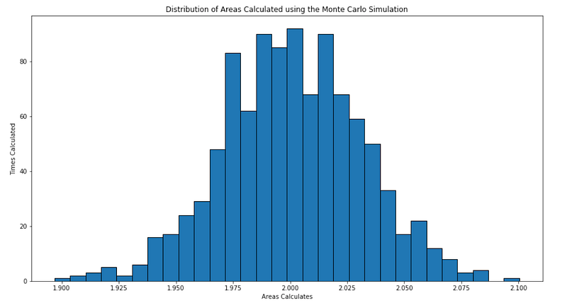
b. Multiple Iterations: Histogram the Distribution

We can create a histogram of the distributions of the areas we are getting, i.e. calculate N areas under the function curve and plot the histogram of each area.

We can see that the mean is at 2, which is our analytical solution, therefore, using the Monte Carlo Method to approximate the analytical solution via a numerical solution yields very similar results asymptotically.

3. Simple Integration using the Estimation of a function

We can also use the estimation of a function method rather than the simple average.

In this example we will use the following integral:

With closed-form solution being:

a. Expressing the Integral as an Expectation

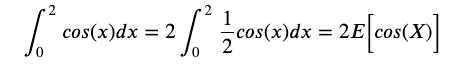
We can re-express the above integral as an expectation as follows:

We can then estimate the value of the integral as a function of sample size. We will be using sample size of 1000, 2000, all the way to 50000 with a step of 1000.

b. Simulating the value of the cos integral

import numpy as np
import matplotlib.pyplot as plt
from scipy.stats import uniform

We can create empty vectors that we can use to store the value of the Monte Carlo estimates and standard deviations, with 50 different sample sizes, ranging from N = 1000 to N = 50000

This will be useful for plotting these values later

In this case, instead of creating an array of N random numbers, we want to increase the size of N from 1000 to 50000, therefore we increase the random numbers in a for loop and with each iteration we multiply N by the iteration index

We are evaluating:

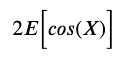
therefore, we need to multiply our cosine function by a factor of 2

c. Plot the estimates against the analytical value of the integral

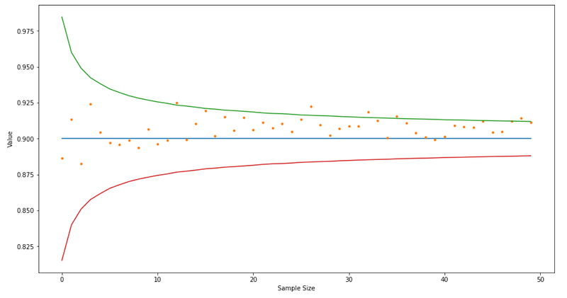
We see a similar result as we did with the plotting of the histogram of the random variables in the previous section. The mean is at 0.900 which is the analytical solution, and the numerical solution asymptotically approximates the actual solution.

This Article is published on The Quant Journey, an initiative started to take the readers along side this journey towards learning about quantitative finance topics.