Trading with MACD and RSI — Yfinance & Python.

#TradersWhoCode

AGENDA:

Installation and Setup
Introduction to Trend and Momentum indicators.
Generate trading signals
Plot Entry/Exit points
Interpret Graphs

Installation & Setup

I am going to assume most people already have python setup but in case you are new to coding, please navigate to the documentation and get your computer ready to go before you continue.

For those of you who have used Python and are comfortable with your setup, you can just import the libraries listed below and skip to the meat of this article.

pip install yfinance

The link below does a great job listing the steps to using the ‘yfinance’ library. (https://algotrading101.com/learn/yfinance-guide/).

Introduction to Momentum trading:

There are 4 main types of technical indicators used when trading stocks while tracking the market.

Trend
Momentum
Volume
Volatility

Most experienced traders come up with their own unique strategy using a combination of these oscillators to implement a game plan for the type of asset they are investing in.

In this article, we will look at the Moving Average Convergence Divergence -which is a trend-following, momentum indicator that shows the relationship between two moving averages of a security’s price. We calculate the MACD by subtracting the 26-week exponential moving average (EMA) from the 12 week EMA period.

We will also look at the Relative Strength Index, which describes a momentum indicator that measures the magnitude of recent price changes in order to evaluate overbought or oversold conditions in the price of a stock or other asset.

Why are these important?

Important for understanding whether the bullish or bearish movement in the price is strengthening or weakening.
Looks at the pace of recent price changes to determine whether a stock is ripe for a rally or a selloff.

import pandas as pd
import numpy as np
import yfinance as yf
import pandas_datareader as pdr
import datetime as dt
import matplotlib.pyplot as plt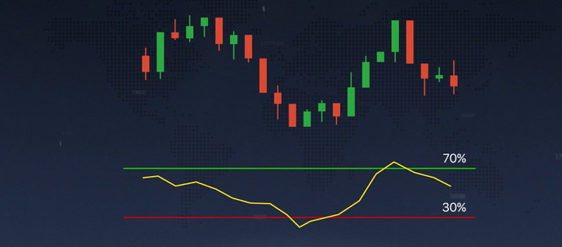

Getting Started!

Let’s begin by selecting the ticker(s) we want to evaluate using Yahoo Finance’s historical data, then set the datetime to today’s date.

ticker = 'FB'

# Last 3 years closing prices starting from Jan 2, 2018.
 
now = dt.datetime.now()
startyear = 2018
startmonth = 1 
startday = 2
start = dt.datetime(startyear, startmonth, startday)

df = pdr.get_data_yahoo(ticker, start, now)

df.tail()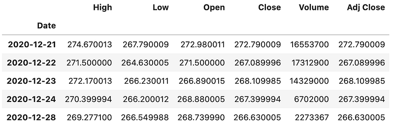

Relative Strength Index (RSI):

When the RSI surpasses the horizontal 30 reference level, it is a bullish sign and when it slides below the horizontal 70 reference level, it is a bearish sign.

## 14_Day RSI

df['Up Move'] = np.nan
df['Down Move'] = np.nan
df['Average Up'] = np.nan
df['Average Down'] = np.nan
# Relative Strength
df['RS'] = np.nan
# Relative Strength Index
df['RSI'] = np.nan

## Calculate Up Move & Down Move

for x in range(1, len(df)):
    df['Up Move'][x] = 0
    df['Down Move'][x] = 0
    
    if df['Adj Close'][x] > df['Adj Close'][x-1]:
        df['Up Move'][x] = df['Adj Close'][x] - df['Adj Close'][x-1]
        
    if df['Adj Close'][x] < df['Adj Close'][x-1]:
        df['Down Move'][x] = abs(df['Adj Close'][x] - df['Adj Close'][x-1])  
        
## Calculate initial Average Up & Down, RS and RSI

df['Average Up'][14] = df['Up Move'][1:15].mean()
df['Average Down'][14] = df['Down Move'][1:15].mean()
df['RS'][14] = df['Average Up'][14] / df['Average Down'][14]
df['RSI'][14] = 100 - (100/(1+df['RS'][14]))

## Calculate rest of Average Up, Average Down, RS, RSI

for x in range(15, len(df)):
    df['Average Up'][x] = (df['Average Up'][x-1]*13+df['Up Move'][x])/14
    df['Average Down'][x] = (df['Average Down'][x-1]*13+df['Down Move'][x])/14
    df['RS'][x] = df['Average Up'][x] / df['Average Down'][x]
    df['RSI'][x] = 100 - (100/(1+df['RS'][x]))

You can ‘print(df)’ to see the DataFrame, it should look like a long table with 6 new columns.

Plot the RSI and ‘Close Prices’ :

## Chart the stock price and RSI

plt.style.use('_classic_test')

fig, axs = plt.subplots(2, sharex=True, figsize=(13,9))
fig.suptitle('Facebook Stock Price (top) - 14 day RSI (bottom)')

axs[0].plot(df['Adj Close'])
axs[1].plot(df['RSI'])
axs[0].grid()
axs[1].grid()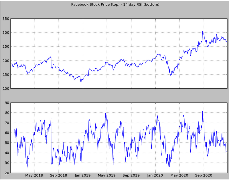

***Please visit my GitHub for a complete list of awesome Font themes and Styles you can use for your graphs! ******

GENERATE BUY & SELL SIGNALS:

## Calculate the buy & sell signals
## Initialize the columns that we need

df['Long Tomorrow'] = np.nan
df['Buy Signal'] = np.nan
df['Sell Signal'] = np.nan
df['Buy RSI'] = np.nan
df['Sell RSI'] = np.nan
df['Strategy'] = np.nan

## Calculate the buy & sell signals

for x in range(15, len(df)):
    
    # Calculate "Long Tomorrow" column
    if ((df['RSI'][x] <= 40) & (df['RSI'][x-1]>40) ):
        df['Long Tomorrow'][x] = True
    elif ((df['Long Tomorrow'][x-1] == True) & (df['RSI'][x] <= 70)):
        df['Long Tomorrow'][x] = True
    else:
        df['Long Tomorrow'][x] = False
        
    # Calculate "Buy Signal" column
    if ((df['Long Tomorrow'][x] == True) & (df['Long Tomorrow'][x-1] == False)):
        df['Buy Signal'][x] = df['Adj Close'][x]
        df['Buy RSI'][x] = df['RSI'][x]
        
    # Calculate "Sell Signal" column
    if ((df['Long Tomorrow'][x] == False) & (df['Long Tomorrow'][x-1] == True)):
        df['Sell Signal'][x] = df['Adj Close'][x]
        df['Sell RSI'][x] = df['RSI'][x]
        
## Calculate strategy performance
df['Strategy'][15] = df['Adj Close'][15]

for x in range(16, len(df)):
    if df['Long Tomorrow'][x-1] == True:
        df['Strategy'][x] = df['Strategy'][x-1]* (df['Adj Close'][x] / df['Adj Close'][x-1])
    else:
        df['Strategy'][x] = df['Strategy'][x-1]

Exit / Entry:

## Chart the buy/sell signals:

plt.style.use('_classic_test')
fig, axs = plt.subplots(2, sharex=True, figsize=(13,9))
fig.suptitle('Stock Price (top) & 14 day RSI (bottom)')

## Chart the stock close price & buy/sell signals:

axs[0].scatter(df.index, df['Buy Signal'],  color = 'green',  marker = '^', alpha = 1)
axs[0].scatter(df.index, df['Sell Signal'],  color = 'red',  marker = 'v', alpha = 1)
axs[0].plot(df['Adj Close'], alpha = 0.8)
axs[0].grid()

## Chart RSI & buy/sell signals:

axs[1].scatter(df.index, df['Buy RSI'],  color = 'green', marker = '^', alpha = 1)
axs[1].scatter(df.index, df['Sell RSI'],  color = 'red', marker = 'v', alpha = 1)
axs[1].plot(df['RSI'], alpha = 0.8)
axs[1].grid()

Moving Average Convergence Divergence (MACD):

## Calculate the MACD and Signal Line indicators
## Calculate the Short Term Exponential Moving Average

ShortEMA = df.Close.ewm(span=12, adjust=False).mean()

## Calculate the Long Term Exponential Moving Average

LongEMA = df.Close.ewm(span=26, adjust=False).mean()

## Calculate the Moving Average Convergence/Divergence (MACD)

MACD = ShortEMA - LongEMA

## Calcualte the signal line
signal = MACD.ewm(span=9, adjust=False).mean()

Plot MACD & Signal Line:

## Plot the Chart

plt.figure(figsize=(14,8))
plt.style.use('classic')

plt.plot(df.index, MACD, label='FB MACD', color = 'blue')
plt.plot(df.index, signal, label='Signal Line', color='red')
plt.xticks(rotation=45)
plt.legend(loc='upper left')
plt.show()

Trading Facebook 3-Year Metrics:

## Performance statistics
## Number of trades

trade_count = df['Buy Signal'].count()

## Average Profit per/trade:

average_profit = ((df['Strategy'][-1] / df['Strategy'][15])**(1/trade_count))-1

## Number of days per/trade

total_days = df['Long Tomorrow'].count()
average_days = int(total_days / trade_count)

print('Strategy yielded ', trade_count, ' trades')
print('Average trade lasted ', average_days, ' days per trade')
print('Our average profit per trade was ', average_profit*100, '%')

Thanks for reading!

If you found this article useful, feel welcome to download my personal codes on GitHub. You can also email me directly at [email protected] and find me on LinkedIn. Interested in learning more about data analytics, data science and machine learning applications? Follow me on Medium.