Modeling the Black-Scholes-Merton (BSM) Model in Python

Creating Python functions to price call and put options and demonstrating with examples.

Introduction

Several Python libraries now include built-in functions for calculating the price of an option using the Black-Scholes-Merton model. These functions, however, are meaningless if the variables that comprise them are not fully understood by the user. It is more difficult to justify the price without knowing the relationships between the variables. In this post, we will quickly define the model’s assumptions, break it down into variables, and code it in Python.

The Black-Scholes-Merton Model: Definition and Assumptions

The Black-Scholes-Merton (BSM) model is an equation used to find the price of a call or put option using specific variables. The model employs probability theory by forecasting the future value using the historical volatility as a predictive component. I discussed volatility in greater depth in my previous post.

The BSM model makes the following assumptions:

1. The volatility is assumed to be constant, meaning that it does not change over time. In the real world, volatility is dynamic and unpredictable;
2. The interest rate, like volatility, is constant and predictable.
3. The model is based on a normal distribution of underlying asset returns, which is synonymous with underlying asset prices being lognormally distributed. The lognormal distribution allows for a stock price distribution ranging from 0 to infinity (no negative prices of the underlying). I covered the principles behind the log returns in this post;
4. Stock moves cannot be predicted, so-called a random walk;
5. During the option’s term, the stock pays no dividend (which, of course, does not always apply to certain stocks in real life);
6. The model is European-style, which means that an option can only be exercised on its expiration date;
7. The model assumes there are no fees for buying and selling options and stocks (this is not the case in the real world), and;
8. The markets are liquid and the options can be bought/sold at any point in time (this does not always hold true in the markets).

The Black-Scholes-Merton Model: The Equation

In general, the model uses five basic inputs to calculate a theoretical value for an option:

1. Strike price
2. Expiration date
3. The current stock price
4. The current risk-free interest rate
5. The stock’s volatility

The fifth output is tricky because the model assumes that volatility is constant, whereas in reality it varies over time. As a result, the theoretical price of the model may not always correspond to the price found in the market.

Now, let’s go over the equations for calculating the fair value of put and call options.

where,

c = call price

p = put price

S = current price of the underlying asset

K = Exercise price

r = Risk free rate of return

T = Remaining time until expiration in years

σ = volatility

It is important to note that the model uses the annualized standard deviation of the stock return as a measure of volatility (σ). Therefore, we need to annualized the standard deviations of log returns. We assume 252 trading days in a year. The formula is as follows:

annualized (σ) = periodic (σ) * square root of 252 days

So, if standard deviation of daily returns were 5%, the annualized volatility equals to 79.4% (0.05 * sqrt[252]).

Some traders use the actual number of calendar days in a year (365). It is simply a preference.

Same applies to time (T) variable since it is calculated in years in the model. If we have a shorter period than a year, we need to identify its proportion to a whole year. Most of the time, the traders work with number of days to expiration. For example, if an option has 31 days to expiration, T equals to 0.12 or 12% (31/252).

Black-Scholes-Merton Model in Python

To model the equation, we are going to need two Python libraries: NumPy and SciPy. Later, we will also use the mathplotlib library to verify our coding. Let’s import them.

import numpy as np
from scipy.stats import norm #importing the normal distribution function only 
import matplotlib.pyplot as plt

The SciPy library is mostly needed to call the normal distribution function into the equation of the BSM model.

N = norm.cdf #defining a normal distribution 

Now, using the BSM model equation from above, let’s write functions to calculate the put and call option prices.

#call price function, sigma=volatility(σ)
def BSM_call_price(S, K , T , r , sigma):
    d1 = (np.log(S/K) + (r + sigma**2/2)*T) / (sigma * np.sqrt(T)) 
    d2 = d1 - sigma * np.sqrt(T)
    return S * N(d1) - K * np.exp(-r*T) * N(d2) 

#put price function, sigma = volatility(σ)
def BSM_put_price(S, K , T , r , sigma):
    d1 = (np.log(S/K) + (r + sigma**2/2)*T) / (sigma * np.sqrt(T))
    d2 = d1 - sigma * np.sqrt(T)
    return K * np.exp(-r*T) * N(-d2) - S * N(-d1)

Okay, the functions are coded. We can now quickly determine whether we did it correctly by observing how option prices react to changes in stock prices. Let’s start by giving the variables some parameters.

K = 50

r = 0.2

T = 1

sigma = 0.5

S = np.arange(25,100) We’ll look at how the option price changes in relation to the stock price as it moves between 25 and 100.

K = 50
r = 0.2
T = 1
sigma = 0.5

S = np.arange(25,100) # stock prices between 25 and 100


calls = []
for s in S: 
  x = BSM_call_price(s, K , T , r ,sigma)
  calls.append(x)

puts = []
for s in S: 
  x = BSM_put_price(s, K , T , r ,sigma)
  puts.append(x)

plt.plot(S,calls, label = 'Call Price')
plt.plot(S,puts, label = 'Put Price')
plt.xlabel('Stock Price')
plt.ylabel('Option Price')
plt.title('Black-Scholes-Merton Model')
plt.legend()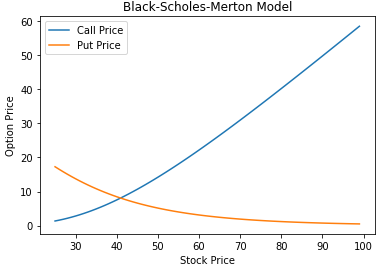

According to the graph above, the call option price rises as the stock price rises, whereas the put option price falls as the stock price rises. It seems like we coded the model correctly.

Finally, let’s compute the call price for a particular SPY strike price and compare it to the market value.

Let’s use the yfinance library to retrieve data on SPY options:

pip install yfinance
import yfinance as yf
SPY= yf.Ticker('SPY')
SPY.options

Randomly, let’s choose the ‘2023–03–31’ call options chain, which expires in 124 days (as of time of writing). The SPY, on 25 November 2022, closed at around USD 402. Let’s see the call options between 400 and 405 strikes.

option = SPY.option_chain('2023-03-31')
option
calls = option.calls

calls[calls['strike'].between(400, 405)]

Since there is no $402 strike we will do the BSM calculation using the $400 strike. Let’s line up our variables:

K = 400

r = 0.0374 (30-year treasury yield)

T = 124/252 = 0.49

S = 402

For the sigma, we can quickly calculate the standard deviation of log returns (year to date) and then annualize it.

import numpy as np
SPY2 = yf.download('SPY', start = '2022-01-01', end = '2022-11-27')
SPY2['pct_change'] = SPY2.Close.pct_change()
SPY2['log_return'] = np.log(1 + SPY2['pct_change'])
std = SPY2['log_return'].std()
annualized_sigma = std * np.sqrt(252)


#returns 0.24689871466473537

We have all variables, let’s plug them into our BSM_call_price function.

BSM_call_price(402, 400, 0.49, 0.0374, annualized_sigma)

#returns 32.07030393549425

The market’s price for the 400-strike call option is $23.15, cheaper by $8.92 from the calculated price by the BSM model. Most of the time, the BSM prices do not match any market, which is primarily due to its assumptions.

Today, traders and investors use the BSM model with a few tweaks, particularly around the volatility and interest rate inputs, to better predict option prices.

Thank you for reading.

If you would like to receive stock market update three times a week, please subscribe to https://szymanskiresearch.substack.com/ . It is free!

Related posts:

Disclaimer: The information contained in this blog post is strictly for educational and entertainment purposes only. This is also not an investment advice. All views expressed in this blog are my own and do not represent the opinions of any entity whatsoever with which I have been, am now, or will be affiliated.

More content at PlainEnglish.io. Sign up for our free weekly newsletter. Follow us on Twitter, LinkedIn, YouTube, and Discord. Interested in Growth Hacking? Check out Circuit.