Summary

This content explains the concepts of Weight of Evidence (WoE) and Information Value (IV) in data science, using the Titanic dataset and Julia programming language.

Abstract

The content discusses how data scientists can use the Weight of Evidence (WoE) and Information Value (IV) concepts to understand the relationships between independent and dependent variables, particularly in classification problems. The author uses the Titanic dataset and Julia programming language to explain and implement these concepts, focusing on the "Survived" and "Sex" variables as examples. The author breaks down the formulas and calculations for WoE and IV, and provides detailed code snippets. The article concludes that WoE can be used for encoding and reducing columns, while IVs offer a basis for further analysis and feature engineering. The author also invites comments on improving their Julia coding skills.

Bullet points

The author is interested in understanding the relationships between independent and dependent variables.
The concepts of Weight of Evidence (WoE) and Information Value (IV) are used to analyze the Titanic dataset using Julia programming language.
WoE is explained as the ratio of proportions of the population in a certain class, and its formula is provided.
The author explains how to calculate WoE using the "Survived" and "Sex" variables as an example.
Code snippets are provided for calculating WoE for "Male" and "Female" classes.
The author explains that IV combines different WoEs for the same independent variable.
The author provides the formula for calculating IV and demonstrates it using the "Sex" variable.
The author provides code snippets for calculating IV for "Male" and "Female" classes and summing them up to obtain the IV for the "Sex" variable.
The author provides a table for IV and its predictive power.
The author explains that WoE is used for encoding and reducing columns, while IVs offer a basis for further analysis and feature engineering.
The author invites comments on improving their Julia coding skills.
The author promotes an AI service that they recommend.

Model? Or do you mean Weight of Evidence (WoE) and Information Value (IV)?

Using Titanic data set to explain and implement both the concepts step-by-step. A great opportunity to also code in Julia!

As a data scientist, I’m always interested to know how certain independent variables, such as occupation, influence the dependent variables, such as income. Specifically, when it comes to classification problems, WoE and IV can tell stories between an independent variable and a dependent variable.

These concepts were developed mainly to answer credit scoring problems, where customers are labelled either ‘good’ or ‘bad’, which is based on them defaulting credit repayment. Their associated variables, such as age, are also recorded.

Now, we are applying these concepts on the Titanic data set.

using DataFrames, CSV
df = DataFrame(CSV.File("train.csv"))
show(describe(df), allcols=true)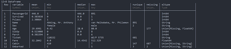

Weight of Evidence (WoE)

The formula of WoE is as such: For each class i of an independent variable x, we want to find the ratio of the proportion/percentage of the population, whose dependent variable y belongs to a certain class, that has the class i, followed by natural log.

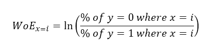
Sound confusing? To put it in context, we can take x as “Sex” and y as “Survived”. “Sex” is divided into 2 classes: “Male” & “Female”. To calculate WoE, 1a. Count the number of perished males (“Sex” = “Male”, “Survived” = 0): 468 1b. Divide the number by the total number of perished passengers (“Survived” = 0): 468/549 = 0.85246 2a. Count the number of surviving males (“Sex” = “Male”, “Survived” = 1): 109 2b. Divide the number by the total number of surviving passengers (“Survived” = 0): 109/342 = 0.31871 3. Divide (1b) result by (2b) result, then take natural log to derive WoE: ln(0.85246/0.31871) = 0.98383

We perform the same steps for “Female” to derive WoE, which is -1.52988. The code is as follows:

survived = by(df, :Survived, (count = :Survived => length))
sex_df = unstack(by(df, [:Sex, :Survived], (count = :Sex => length)), :Sex, :count)

male_event = sex_df[(sex_df.Survived .== 1), :male] / survived[(survived.Survived .== 1), :count]
male_non_event = sex_df[(sex_df.Survived .== 0), :male] / survived[(survived.Survived .== 0), :count]
woe_male = log(male_non_event/male_event)

female_event = sex_df[(sex_df.Survived .== 1), :female] / survived[(survived.Survived .== 1), :count]
female_non_event = sex_df[(sex_df.Survived .== 0), :female] / survived[(survived.Survived .== 0), :count]
woe_female = log(female_non_event/female_event)

Going back to the formula, WoE, through the sign (+/-), shed light on the proportion of male survivors vs the proportion of male victims during the fateful event. However, we are more interested to know the relationship between an independent variable (“Sex”) and a dependent variable (“Survived”).

Information Value (IV)

This will then be able to combine different WoEs for under the same independent variable together. The formula is as such:

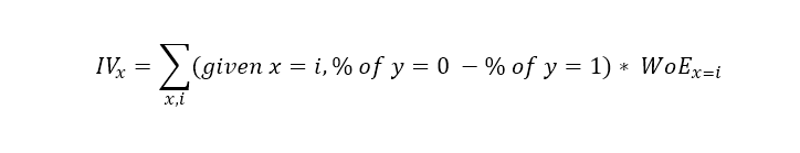
Continuing from our previous example, these are the steps to be taken: 4a. Take the difference between (1b) result and (2b) result: 0.85246 - 0.31871 = 0.53375 4b. Multiply (4a) result with (3) result, which is the WoE: 0.53375 * 0.98383 = 0.52512

We perform the same steps for “Female” and derive 0.81656. Summing both values up, we obtain IV = 1.34168 for the independent variable “Sex”. The code is as follows:

iv_male = (male_non_event - male_event) * woe_male
iv_female = (female_non_event - female_event) * woe_female
iv = iv_male + iv_female

Once we have the IV of the variable, we can check against this table to see the predictive power of the variable. As you can see, the table is saying the variable “Sex” is too good to be true!

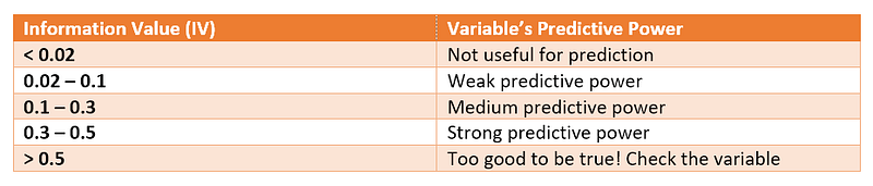
IV table for variable’s predictive power

There are a few assumptions we are making here: firstly, the table serves as a guide when the methodology is created to address credit default problem statement. During that time, the researchers wanted to understand the variables that were likely to influence clients’ credit ratings. The researchers found that the table was very relevant to their problem statement. It was then served as a guide.

Secondly, it has been shown that more females than males survived from the sinking of Titanic. The odds of females surviving is higher than that of males from the accident. Hence, it is no surprise that the variable “Sex” is indeed an exceptional strong predictive power.

Okay, what’s next?

Apart from applying the concepts for research purposes, the main practical use of WoE is for encoding, where you can replace the classes with their associated values. For example, in our example, you can replace “Male” with 0.98383 and “Female” with -1.52988. The reason is obvious: Machine Learning algorithms are primarily taking numbers as inputs, so we have to turn strings to figures before training a model.

Another positive outcome of using WoE is to reduce the number of columns of the input used for training a model. Imagine you have a categorical variable with 10 different classes and you perform a one-hot encoding, you will end up with 10 columns with mostly ‘0’ as values. Using WoE technique, the classes are replaced by their associated WoE values.

As for IVs, they provide a basis for us to drill down further in our relationship analysis between independent and dependent variables. Furthermore, if the variable is a qualitative type, we can use binning method followed by WoE and IV concepts to engineer meaningful features.

That’s all for the explanation for now. Do drop me comments if there is any way I can improve my Julia coding skill, as I recently picked this language up. Cheers!