ML Tutorial 3 — Exploring Regression Techniques and Algorithms

Learn how to perform regression analysis using various algorithms.

Table of Contents 1. Introduction 2. What is Regression Analysis? 3. Types of Regression Techniques 4. Linear Regression 5. Logistic Regression 6. Polynomial Regression 7. Ridge Regression 8. Lasso Regression 9. Elastic Net Regression 10. Support Vector Regression 11. Decision Tree Regression 12. Random Forest Regression 13. Gradient Boosting Regression 14. Neural Network Regression 15. Conclusion

Subscribe for FREE to get your 42 pages e-book: Data Science | The Comprehensive Handbook

Get step-by-step e-books on Python, ML, DL, and LLMs.

1. Introduction

In this tutorial, you will learn how to perform regression analysis using various algorithms. Regression analysis is a powerful technique for modeling the relationship between a dependent variable and one or more independent variables. Regression analysis can help you understand how the changes in the independent variables affect the dependent variable, and also provide predictions based on the data.

There are many types of regression techniques, each with its own advantages and disadvantages. Some of the most common regression techniques are:

Linear regression: This is the simplest and most widely used regression technique. It assumes that the relationship between the dependent and independent variables is linear, and tries to find the best-fitting straight line that minimizes the sum of squared errors.
Logistic regression: This is a special type of regression technique that is used for binary classification problems. It assumes that the dependent variable is a categorical variable that can take only two values, such as 0 or 1, yes or no, etc. It tries to find the best-fitting logistic curve that maximizes the likelihood of the data.
Polynomial regression: This is a generalization of linear regression that allows for nonlinear relationships between the dependent and independent variables. It tries to find the best-fitting polynomial curve that minimizes the sum of squared errors.
Ridge regression: This is a variation of linear regression that adds a regularization term to the cost function. This term penalizes the model for having large coefficients, and helps to reduce overfitting and multicollinearity.
Lasso regression: This is another variation of linear regression that also adds a regularization term to the cost function. However, this term uses the absolute value of the coefficients instead of the square, and helps to perform feature selection by shrinking some coefficients to zero.
Elastic net regression: This is a combination of ridge and lasso regression that uses both the square and the absolute value of the coefficients as regularization terms. This allows for a balance between ridge and lasso regression, and can handle both overfitting and feature selection.
Support vector regression: This is a machine learning technique that is based on the concept of support vector machines. It tries to find the best-fitting hyperplane that has the maximum margin from the data points, and can handle nonlinear and high-dimensional data.
Decision tree regression: This is another machine learning technique that is based on the concept of decision trees. It tries to find the best-fitting tree structure that splits the data into homogeneous regions, and can handle nonlinear and categorical data.
Random forest regression: This is an ensemble technique that combines multiple decision tree regressors and averages their predictions. It tries to improve the accuracy and reduce the variance of the decision tree regression, and can handle nonlinear and high-dimensional data.
Gradient boosting regression: This is another ensemble technique that combines multiple weak regressors and boosts their performance by learning from the errors of the previous regressors. It tries to minimize the loss function by using gradient descent, and can handle nonlinear and high-dimensional data.
Neural network regression: This is a deep learning technique that is based on the concept of artificial neural networks. It tries to find the best-fitting network structure that learns the complex patterns and features from the data, and can handle nonlinear and high-dimensional data.

In this tutorial, you will learn how to implement each of these regression techniques using Python. You will use the popular libraries such as NumPy, Pandas, Scikit-learn, TensorFlow, and Keras to perform the data manipulation, model building, and evaluation. You will also use some sample datasets to demonstrate the application of each technique.

By the end of this tutorial, you will have a solid understanding of the theory and practice of regression analysis, and be able to apply it to your own data problems.

2. What is Regression Analysis?

Regression analysis is a statistical technique that aims to model the relationship between a dependent variable and one or more independent variables. The dependent variable is the variable that you want to explain or predict, while the independent variables are the variables that you use to explain or predict the dependent variable.

For example, suppose you want to study how the price of a house depends on various factors, such as the size, the location, the number of rooms, the age, etc. In this case, the price of the house is the dependent variable, and the factors are the independent variables. Regression analysis can help you find out how each factor affects the price, and also provide an equation that can estimate the price based on the values of the factors.

There are many benefits of using regression analysis, such as:

Understanding the relationship: Regression analysis can help you understand how the dependent and independent variables are related, and whether the relationship is linear, nonlinear, positive, negative, or complex.
Testing hypotheses: Regression analysis can help you test hypotheses about the significance and direction of the relationship, and whether the relationship is causal or correlational.
Estimating the value: Regression analysis can help you estimate the value of the dependent variable based on the values of the independent variables, and also provide a confidence interval and an error term for the estimation.
Optimizing the performance: Regression analysis can help you optimize the performance of a system or a process by finding the optimal values of the independent variables that maximize or minimize the value of the dependent variable.
Forecasting the future: Regression analysis can help you forecast the future value of the dependent variable based on the historical data and the trends of the independent variables.

In the next section, you will learn about the different types of regression techniques and how to choose the best one for your data problem.

3. Types of Regression Techniques

There are many types of regression techniques, each with its own assumptions, advantages, and disadvantages. Choosing the best regression technique for your data problem depends on several factors, such as:

The type and shape of the data: You need to consider the type and shape of the data, such as whether the data is continuous or categorical, linear or nonlinear, normal or skewed, etc. Some regression techniques can handle only certain types of data, while others can handle more general types of data.
The number and nature of the variables: You need to consider the number and nature of the variables, such as whether there is one or more independent variables, whether the variables are correlated or independent, whether the variables are relevant or irrelevant, etc. Some regression techniques can handle only a single independent variable, while others can handle multiple independent variables. Some regression techniques can also perform feature selection or regularization to deal with multicollinearity or overfitting.
The goal and objective of the analysis: You need to consider the goal and objective of the analysis, such as whether you want to understand the relationship, test hypotheses, estimate the value, optimize the performance, or forecast the future. Some regression techniques can provide more interpretability and explanation, while others can provide more accuracy and prediction.

In general, there are two main categories of regression techniques: parametric and non-parametric.

Parametric regression techniques assume that the data follows a certain distribution or function, and try to find the best-fitting parameters that describe the relationship. Parametric regression techniques are usually simpler and faster, but they may not fit the data well if the assumptions are violated. Some examples of parametric regression techniques are linear regression, logistic regression, polynomial regression, ridge regression, lasso regression, and elastic net regression.

Non-parametric regression techniques do not assume that the data follows a certain distribution or function, and try to find the best-fitting model that adapts to the data. Non-parametric regression techniques are usually more flexible and robust, but they may be more complex and computationally intensive. Some examples of non-parametric regression techniques are support vector regression, decision tree regression, random forest regression, gradient boosting regression, and neural network regression.

In the following sections, you will learn how to implement each of these regression techniques using Python, and compare their performance on some sample datasets.

4. Linear Regression

Linear regression is one of the simplest and most widely used regression techniques. It assumes that the relationship between the dependent and independent variables is linear, and tries to find the best-fitting straight line that minimizes the sum of squared errors.

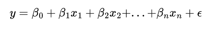
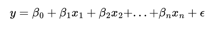
The equation of a linear regression model is:

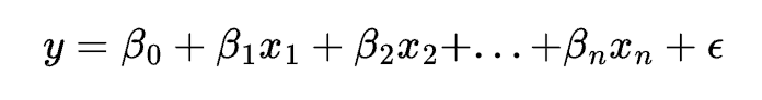
where y is the dependent variable, x1, x2, …, xn are the independent variables, \beta0, \beta1, …, \betan are the coefficients, and \epsilon is the error term.

The coefficients represent the slope of the line, and the error term represents the deviation of the actual value from the predicted value. The goal of linear regression is to find the optimal values of the coefficients that minimize the sum of squared errors, which is also called the cost function or the loss function.

There are different methods to estimate the coefficients, such as the ordinary least squares (OLS) method, the gradient descent method, the normal equation method, etc. In this tutorial, you will use the OLS method, which is the most common and simple method. The OLS method calculates the coefficients by solving a system of linear equations, which can be written as:

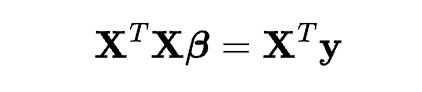
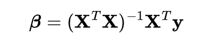
where \mathbf{X} is the matrix of the independent variables, \mathbf{y} is the vector of the dependent variable, and {\beta} is the vector of the coefficients. The solution for the coefficients is:

To implement linear regression using Python, you will use the NumPy library, which is a popular library for scientific computing. NumPy provides various functions and methods for working with arrays and matrices, such as creating, manipulating, and performing operations on them. You will also use the Pandas library, which is a popular library for data analysis. Pandas provides various functions and methods for working with data structures and formats, such as reading, writing, and processing data.

In the next section, you will see an example of how to perform linear regression on a sample dataset using Python.

5. Logistic Regression

Logistic regression is a special type of regression technique that is used for binary classification problems. It assumes that the dependent variable is a categorical variable that can take only two values, such as 0 or 1, yes or no, etc. It tries to find the best-fitting logistic curve that maximizes the likelihood of the data.

The equation of a logistic regression model is:

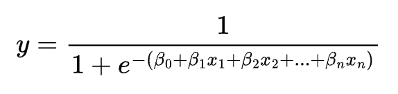
where y is the probability of the dependent variable being 1, x1, x2, …, xn are the independent variables, \beta0, \beta1, …, \betan are the coefficients, and e is the base of the natural logarithm.

The coefficients represent the log-odds of the dependent variable being 1, and the logistic function maps the log-odds to a probability between 0 and 1. The goal of logistic regression is to find the optimal values of the coefficients that maximize the likelihood function, which is the product of the probabilities of the observed outcomes.

There are different methods to estimate the coefficients, such as the maximum likelihood estimation (MLE) method, the gradient descent method, the Newton-Raphson method, etc. In this tutorial, you will use the MLE method, which is the most common and simple method. The MLE method calculates the coefficients by iteratively updating them until the likelihood function reaches its maximum value, which can be written as:

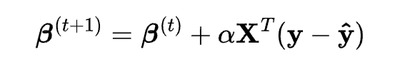
where {\beta}^{(t)} is the vector of the coefficients at iteration t, \alpha is the learning rate, \mathbf{X} is the matrix of the independent variables, \mathbf{y} is the vector of the actual outcomes, and \mathbf{\hat{y}} is the vector of the predicted outcomes.

To implement logistic regression using Python, you will use the Scikit-learn library, which is a popular library for machine learning. Scikit-learn provides various functions and methods for building, training, and evaluating machine learning models, such as logistic regression. You will also use the NumPy and Pandas libraries, which you have already learned in the previous section.

In the next section, you will see an example of how to perform logistic regression on a sample dataset using Python.

6. Polynomial Regression

Polynomial regression is a generalization of linear regression that allows for nonlinear relationships between the dependent and independent variables. It tries to find the best-fitting polynomial curve that minimizes the sum of squared errors.

The equation of a polynomial regression model is:

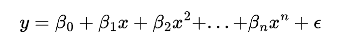
where y is the dependent variable, x is the independent variable, \beta0, \beta1, …, \betan are the coefficients, n is the degree of the polynomial, and \epsilon is the error term.

The coefficients represent the weights of the polynomial terms, and the error term represents the deviation of the actual value from the predicted value. The goal of polynomial regression is to find the optimal values of the coefficients that minimize the sum of squared errors, which is the same as the linear regression.

However, unlike linear regression, polynomial regression can handle nonlinear relationships by adding higher-order terms to the model. The degree of the polynomial determines the complexity and flexibility of the model. A higher degree can fit the data better, but it may also cause overfitting and high variance. A lower degree can prevent overfitting, but it may also cause underfitting and high bias. Therefore, choosing the optimal degree of the polynomial is a trade-off between bias and variance, and it depends on the data and the problem.

To implement polynomial regression using Python, you will use the Scikit-learn library, which you have already learned in the previous section. Scikit-learn provides a function called PolynomialFeatures, which can generate polynomial and interaction features from the original features. You will also use the NumPy and Pandas libraries, which you have already learned in the previous section.

In the next section, you will see an example of how to perform polynomial regression on a sample dataset using Python.

7. Ridge Regression

Ridge regression is a variation of linear regression that adds a regularization term to the cost function. This term penalizes the model for having large coefficients, and helps to reduce overfitting and multicollinearity.

The equation of a ridge regression model is:

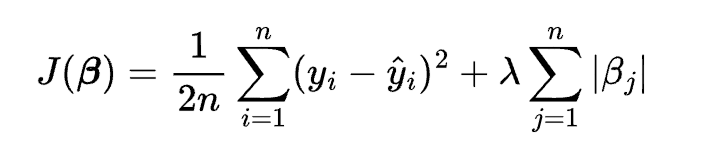
where y is the dependent variable, x1, x2, …, xn are the independent variables, \beta0, \beta1, …, \betan are the coefficients, and \epsilon is the error term. The cost function of ridge regression is:

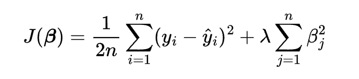
where n is the number of observations, yi is the actual value of the dependent variable for the i-th observation, \hat{y}i is the predicted value of the dependent variable for the i-th observation, \lambda is the regularization parameter, and \betaj is the coefficient for the j-th independent variable.

To implement ridge regression using Python, you will use the Scikit-learn library, which you have already learned in the previous section. Scikit-learn provides a class called Ridge, which can fit a ridge regression model and provide various methods for evaluation and prediction. You will also use the NumPy and Pandas libraries, which you have already learned in the previous section.

In the next section, you will see an example of how to perform ridge regression on a sample dataset using Python.

8. Lasso Regression

Lasso regression is another variation of linear regression that also adds a regularization term to the cost function. However, this term uses the absolute value of the coefficients instead of the square, and helps to perform feature selection by shrinking some coefficients to zero.

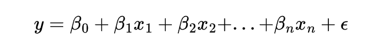
The equation of a lasso regression model is:

To implement lasso regression using Python, you will use the Scikit-learn library, which you have already learned in the previous section. Scikit-learn provides a class called Lasso, which can fit a lasso regression model and provide various methods for evaluation and prediction. You will also use the NumPy and Pandas libraries, which you have already learned in the previous section.

In the next section, you will see an example of how to perform lasso regression on a sample dataset using Python.

9. Elastic Net Regression

Elastic net regression is a combination of ridge and lasso regression that uses both the square and the absolute value of the coefficients as regularization terms. This allows for a balance between ridge and lasso regression, and can handle both overfitting and feature selection.

The equation of an elastic net regression model is:

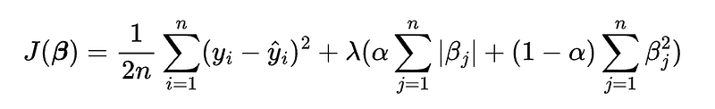
where n is the number of observations, yi is the actual value of the dependent variable for the i-th observation, \hat{y}i is the predicted value of the dependent variable for the i-th observation, \lambda is the regularization parameter, \alpha is the mixing parameter, and \betaj is the coefficient for the j-th independent variable.

The regularization parameter \lambda controls the strength of the penalty. A higher \lambda means a stronger penalty, which shrinks the coefficients more and reduces the variance and the number of features of the model. A lower \lambda means a weaker penalty, which shrinks the coefficients less and reduces the bias and the sparsity of the model. The mixing parameter \alpha controls the balance between ridge and lasso regression. A higher \alpha means more lasso-like behavior, which favors sparse solutions and feature selection. A lower \alpha means more ridge-like behavior, which favors dense solutions and regularization. Therefore, choosing the optimal values of \lambda and \alpha is a trade-off between bias and variance, and it depends on the data and the problem.

To implement elastic net regression using Python, you will use the Scikit-learn library, which you have already learned in the previous section. Scikit-learn provides a class called ElasticNet, which can fit an elastic net regression model and provide various methods for evaluation and prediction. You will also use the NumPy and Pandas libraries, which you have already learned in the previous section.

In the next section, you will see an example of how to perform elastic net regression on a sample dataset using Python.

10. Support Vector Regression

Support vector regression is a machine learning technique that is based on the concept of support vector machines. It tries to find the best-fitting hyperplane that has the maximum margin from the data points, and can handle nonlinear and high-dimensional data.

The equation of a support vector regression model is:

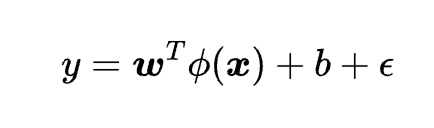
where y is the dependent variable, {x} is the independent variable, {w} is the weight vector, b is the bias term, \phi is the feature mapping function, and \epsilon is the error term. The cost function of support vector regression is:

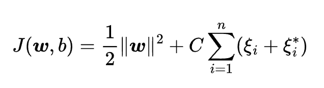
where n is the number of observations, C is the regularization parameter, \xii and \xii* are the slack variables that measure the deviation of the data points from the hyperplane. The goal of support vector regression is to find the optimal values of {w} and b that minimize the cost function, subject to the constraints:

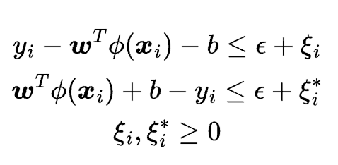
where yi is the actual value of the dependent variable for the i-th observation, and {x}i is the independent variable for the i-th observation. The regularization parameter C controls the trade-off between the complexity and the accuracy of the model. A higher C means a smaller margin and a lower error, but it may also cause overfitting and high variance. A lower C means a larger margin and a higher error, but it may also prevent overfitting and reduce the variance. The feature mapping function \phi transforms the original features into a higher-dimensional space, where the data points can be more easily separated by a linear hyperplane. However, computing \phi explicitly can be very expensive and impractical, especially for high-dimensional data. Therefore, support vector regression uses a kernel function K, which can compute the inner product of the mapped features without explicitly mapping them. The kernel function K is defined as:

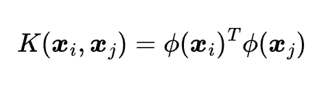
where {x}i and {x}j are any two independent variables. There are many types of kernel functions, such as linear, polynomial, radial basis function, sigmoid, etc. Choosing the best kernel function for your data problem depends on the characteristics and the distribution of the data.

To implement support vector regression using Python, you will use the Scikit-learn library, which you have already learned in the previous section. Scikit-learn provides a class called SVR, which can fit a support vector regression model and provide various methods for evaluation and prediction. You will also use the NumPy and Pandas libraries, which you have already learned in the previous section.

In the next section, you will see an example of how to perform support vector regression on a sample dataset using Python.

11. Decision Tree Regression

Decision tree regression is another machine learning technique that is based on the concept of decision trees. It tries to find the best-fitting tree structure that splits the data into homogeneous regions, and can handle nonlinear and categorical data.

The equation of a decision tree regression model is:

where y is the dependent variable, {x} is the independent variable, and f is the function that maps the independent variable to the dependent variable. The function f is defined by a tree structure, which consists of nodes and branches. Each node represents a test or a condition on an independent variable, and each branch represents an outcome or a decision. The tree starts with a root node, which is the first node that splits the data. The tree ends with leaf nodes, which are the final nodes that assign a value to the dependent variable. The goal of decision tree regression is to find the optimal tree structure that minimizes the impurity or the variance of the data in each leaf node.

To implement decision tree regression using Python, you will use the Scikit-learn library, which you have already learned in the previous section. Scikit-learn provides a class called DecisionTreeRegressor, which can fit a decision tree regression model and provide various methods for evaluation and prediction. You will also use the NumPy and Pandas libraries, which you have already learned in the previous section.

In the next section, you will see an example of how to perform decision tree regression on a sample dataset using Python.

12. Random Forest Regression

Random forest regression is an ensemble technique that combines multiple decision tree regressors and averages their predictions. It tries to improve the accuracy and reduce the variance of the decision tree regression, and can handle nonlinear and high-dimensional data.

The equation of a random forest regression model is:

where y is the dependent variable, {x} is the independent variable, M is the number of decision tree regressors, and fm is the function that maps the independent variable to the dependent variable for the m-th decision tree regressor. The goal of random forest regression is to find the optimal values of fm for each decision tree regressor that minimize the mean squared error of the prediction, and then average their predictions to obtain the final output.

To implement random forest regression using Python, you will use the Scikit-learn library, which you have already learned in the previous section. Scikit-learn provides a class called RandomForestRegressor, which can fit a random forest regression model and provide various methods for evaluation and prediction. You will also use the NumPy and Pandas libraries, which you have already learned in the previous section.

In the next section, you will see an example of how to perform random forest regression on a sample dataset using Python.

13. Gradient Boosting Regression

Gradient boosting regression is another ensemble technique that combines multiple weak regressors and boosts their performance by learning from the errors of the previous regressors. It tries to minimize the loss function by using gradient descent, and can handle nonlinear and high-dimensional data.

The equation of a gradient boosting regression model is:

where y is the dependent variable, {x} is the independent variable, M is the number of weak regressors, \alpham is the learning rate for the m-th weak regressor, and fm is the function that maps the independent variable to the dependent variable for the m-th weak regressor. The goal of gradient boosting regression is to find the optimal values of \alpham and fm for each weak regressor that minimize the loss function, which is usually the mean squared error of the prediction. The algorithm of gradient boosting regression is as follows:

Initialize the model with a constant value, such as the mean of the dependent variable.
For each iteration m from 1 to M:

Compute the negative gradient of the loss function with respect to the prediction for each observation, which is also called the pseudo-residual.
Fit a weak regressor, such as a decision tree, to the pseudo-residuals, and obtain the predicted values.
Update the model by adding the product of the learning rate and the predicted values of the weak regressor.

3. Return the final model as the sum of the weak regressors.

To implement gradient boosting regression using Python, you will use the Scikit-learn library, which you have already learned in the previous section. Scikit-learn provides a class called GradientBoostingRegressor, which can fit a gradient boosting regression model and provide various methods for evaluation and prediction. You will also use the NumPy and Pandas libraries, which you have already learned in the previous section.

In the next section, you will see an example of how to perform gradient boosting regression on a sample dataset using Python.

14. Neural Network Regression

Neural network regression is a deep learning technique that is based on the concept of artificial neural networks. It tries to find the best-fitting network structure that learns the complex patterns and features from the data, and can handle nonlinear and high-dimensional data.

The equation of a neural network regression model is:

where y is the dependent variable, {x} is the independent variable, {\theta} is the parameter vector, and f is the function that maps the independent variable to the dependent variable. The function f is defined by a network structure, which consists of layers and units. Each layer is composed of multiple units, and each unit performs a linear or nonlinear transformation on its inputs. The network starts with an input layer, which receives the independent variable. The network ends with an output layer, which produces the dependent variable. The network may also have one or more hidden layers, which process the intermediate outputs of the previous layers. The goal of neural network regression is to find the optimal values of {\theta} that minimize the loss function, which is usually the mean squared error of the prediction. The algorithm of neural network regression is as follows:

Initialize the network structure and the parameter vector randomly.
For each iteration or epoch:

Feed the independent variable to the input layer, and propagate it forward through the network, until the output layer produces the predicted value of the dependent variable.
Compute the error or the difference between the predicted and the actual value of the dependent variable, and propagate it backward through the network, until the input layer receives the error signal.
Update the parameter vector by using gradient descent or other optimization methods, based on the error signal and the learning rate.

3. Return the final network structure and the parameter vector as the model.

To implement neural network regression using Python, you will use the TensorFlow and Keras libraries, which are popular frameworks for building and training deep learning models. TensorFlow provides low-level operations and functions for creating and manipulating tensors, which are multi-dimensional arrays of data. Keras provides high-level APIs and classes for defining and compiling neural network models, and also provides various methods for evaluation and prediction. You will also use the NumPy and Pandas libraries, which you have already learned in the previous section.

In the next section, you will see an example of how to perform neural network regression on a sample dataset using Python.

15. Conclusion

In this tutorial, you have learned how to perform regression analysis using various algorithms. You have seen how to implement each of these algorithms using Python, and how to compare their performance on some sample datasets. You have also learned about the advantages and disadvantages of each algorithm, and how to choose the best one for your data problem.

Regression analysis is a powerful technique for modeling the relationship between a dependent variable and one or more independent variables. It can help you understand how the changes in the independent variables affect the dependent variable, and also provide predictions based on the data. There are many types of regression techniques, each with its own assumptions, advantages, and disadvantages. Choosing the best regression technique for your data problem depends on several factors, such as the type and shape of the data, the number and nature of the variables, and the goal and objective of the analysis.

We hope that this tutorial has been helpful and informative for you. If you have any questions or feedback, please feel free to leave a comment below. Thank you for reading and happy learning!

Subscribe for FREE to get your 42 pages e-book: Data Science | The Comprehensive Handbook

Get step-by-step e-books on Python, ML, DL, and LLMs.