Maximizing Pandas Efficiency: Top 10 Mistakes to Steer Clear of in Your Code
Pandas is a powerful and popular data analysis library in Python, widely used by data scientists and analysts to manipulate and transform data. However, with great power comes great responsibility, and it’s easy to fall into common pitfalls that can lead to inefficient code and slow performance.
In this article, we’ll explore the top 10 mistakes to steer clear of when using Pandas, so you can maximize your efficiency and get the most out of this powerful library. Whether you’re a beginner or a seasoned Pandas user, these tips will help you write better code and avoid common mistakes that can slow you down.

Table of Content:
- Having Column Names with Spaces
- Not Using Query Method for Filtering
- Not using @ Symbol when Writing Complex Queries
- Iterating over Dataframe instead of using Vectorization
- Treating Slices of Dataframe as New Dataframe
- Not Using Chain Commands for Multiple Trasnofrations
- Not Setting Column dtypes Correctly
- Not Using Pandas Plotting Builtin Function
- Aggregation manually instead of using .groupby()
- Saving Large Datasets as CSV File
If you want to study Data Science and Machine Learning for free, check out these resources:
- Free interactive roadmaps to learn Data Science and Machine Learning by yourself. Start here: https://aigents.co/learn/roadmaps/intro
- The search engine for Data Science learning resources (FREE). Bookmark your favorite resources, mark articles as complete, and add study notes. https://aigents.co/learn
- Want to learn Data Science from scratch with the support of a mentor and a learning community? Join this Study Circle for free: https://community.aigents.co/spaces/9010170/
If you want to start a career in data science & AI and do not know how. I offer data science mentoring sessions and long-term career mentoring:
- Long-term mentoring: https://lnkd.in/dtdUYBrM
- Mentoring sessions: https://lnkd.in/dXeg3KPW
Join the Medium membership program for only 5$ to continue learning without limits. I’ll receive a small portion of your membership fee if you use the following link, at no extra cost to you.
1. Having Column Names with Spaces
Having column names with spaces in Pandas can lead to issues when manipulating data or trying to access column values. When a column name contains a space, it needs to be enclosed in quotes or backticks every time it’s referenced in the code, which can be cumbersome and error-prone. Additionally, you will not be able to use the dot function in pandas, Here’s an example of how having a column name with a space can cause issues in Pandas:
For example, if you have a dataframe with a column name containing a space, say “Sales Amount”, you cannot reference the column using the usual dot notation, like this:
df.Sales Amount
This will result in a syntax error, as the space in the column name causes confusion to Python’s syntax parser.
Instead, you would need to reference the column name using square brackets and quotes, like this:
df['Sales Amount']However, this can be cumbersome and error-prone, especially if you have a lot of column names with spaces.
Another issue with spaces in column names is that some functions in pandas might not be able to handle them properly. For example, if you want to group by a column with a space in the name, like this:
df.groupby('Sales Amount')['Quantity'].sum()You will get a KeyError, as pandas cannot recognize the column name with the space.
To avoid these issues, it’s best to avoid spaces in column names altogether when working with pandas dataframes. Instead, you can use underscores or camelCase to separate words in column names. For example, “Sales_Amount” or “salesAmount”.
2. Not Using Query Method for Filtering
The second mistake you should avoid is not using the query method when filtering the data. The query() method in pandas is a useful tool for creating subsets of a dataframe based on specific conditions. It allows you to filter rows based on a boolean expression that you provide and can be a convenient way to create complex subsets without needing to chain multiple conditions together.
Here’s an example of how to use the query() method to create a subset of a dataframe:
import pandas as pd

df = pd.DataFrame({'name': ['Alice', 'Bob', 'Charlie', 'David'],
                   'age': [25, 30, 35, 40]})

# Subset where age is greater than 30
subset = df.query('age > 30')
In this example, the query() method is used to create a subset of the dataframe df where the age column is greater than 30. The resulting subset is stored in the variable subset.
You can also use the query() method to create subsets based on multiple conditions:
# Subset where age is between 30 and 40, inclusive
subset = df.query('age >= 30 and age <= 40')
In this example, the query() method is used to create a subset of the dataframe df where the age column is between 30 and 40, inclusive.
While the query() method can be a powerful tool, it's important to keep in mind that it can be slower than other methods like boolean indexing or the loc and iloc indexers. Additionally, it's important to be careful with variable scoping and name collisions when using query(). Therefore, it's recommended to use query() judiciously and to consider other methods when appropriate.
3. Not using @ Symbol when Writing Complex Queries
When using the query() method in pandas, it's important to keep in mind that using a string for the query expression may not always be the most efficient or readable approach, especially for complex queries.
An alternative approach is to use the @ symbol to reference variables in the query expression, allowing you to write more readable and flexible code.
Here’s an example of how to use the @ symbol with the query() method:
import pandas as pd

df = pd.read_csv('sales_data.csv')

product_category = 'Electronics'
start_date = '2022-01-01'
end_date = '2022-03-01'
min_sales_amount = 1000
min_quantity = 10

subset = df.query('product_category == @product_category and @start_date <= order_date <= @end_date and (sales_amount >= @min_sales_amount or quantity >= @min_quantity)')
In this example, the @ symbol is used to reference variables in the query expression, making the code more flexible and readable. The variables product_category, start_date, end_date, min_sales_amount, and min_quantity are defined earlier in the code and can be easily modified without needing to update the string expression.
By using the @ symbol to reference variables, you can write more concise and readable queries without sacrificing performance or readability. This approach is especially useful for complex queries involving multiple variables or conditions.
4. Iterating over Dataframe instead of using Vectorization
Vectorization is a powerful technique in data analysis that involves performing operations on entire arrays or columns of data at once, rather than using loops to iterate over each individual element. Using vectorization can often lead to much faster and more efficient code, particularly when working with large datasets.
To illustrate how to use vectorization instead of looping over a data frame, let’s consider a simple example. Suppose we have a data frame with two columns, “x” and “y”, and we want to create a new column “z” that contains the product of “x” and “y”.
Here’s an example of how we might do this using a loop:
import pandas as pd

df = pd.DataFrame({'x': [1, 2, 3], 'y': [4, 5, 6]})

for index, row in df.iterrows():
    df.loc[index, 'z'] = row['x'] * row['y']
This code iterates over each row of the data frame and calculates the product of “x” and “y” for that row, then stores the result in the new “z” column. While this code works, it can be slow and inefficient, particularly for large data frames.
Instead, we can use vectorization to perform this calculation much more efficiently. Here’s an example:
import pandas as pd

df = pd.DataFrame({'x': [1, 2, 3], 'y': [4, 5, 6]})

df['z'] = df['x'] * df['y']
In this code, we simply use the “*” operator to multiply the “x” and “y” columns together and then assign the result to the new “z” column. This code performs the calculation much more efficiently than the loop-based approach.
5. Treating Slices of Dataframe as New Dataframe
When you create a new DataFrame from a slice of an existing DataFrame in pandas, it’s important to note that the new DataFrame is actually a view of the original data, rather than a copy. This means that any changes you make to the new DataFrame will also be reflected in the original DataFrame.
To avoid this behavior and ensure that any edits you make to the new DataFrame do not affect the original DataFrame, you can use the “copy” method to create a copy of the DataFrame. Here’s an example:
import pandas as pd

# Create a sample DataFrame
data = {'name': ['Alice', 'Bob', 'Charlie', 'David', 'Emily'],
        'age': [25, 32, 18, 47, 29],
        'gender': ['F', 'M', 'M', 'M', 'F']}
df = pd.DataFrame(data)

# Create a copy of the DataFrame
new_df = df.loc[df['age'] > 30, ['name', 'age']].copy()

# Modify the new DataFrame
new_df['age'] = new_df['age'] + 5

# Print both DataFrames
print(df)
print(new_df)
In this example, we first create a sample DataFrame with three columns: “name”, “age”, and “gender”. We then select a slice of the DataFrame using the “.loc” indexer to select only the rows where the “age” column is greater than 30, and only the “name” and “age” columns. We then use the “copy” method to create a new DataFrame that is a copy of the slice, rather than a view of the original data.
We then modify the “age” column of the new DataFrame by adding 5 to each value. Because we used the “copy” method to create the new DataFrame, this modification does not affect the original DataFrame.
Finally, we print both DataFrames to confirm that the modification only applies to the new DataFrame, and not the original DataFrame.
6. Not Using Chain Commands for Multiple Trasnofrations
The sixth mistake you need to avoid is creating multiple intermediate dataframes when doing multiple transformations. Instead, it is better to write the transformation in chain commands where all transformations are applied once.
In pandas, you can chain multiple transformations together in a single statement, which can be a more concise and efficient way of applying multiple transformations to a DataFrame. Here’s an example of how to transform a DataFrame using chain commands:
import pandas as pd

# Create a sample DataFrame
data = {'name': ['Alice', 'Bob', 'Charlie', 'David', 'Emily'],
        'age': [25, 32, 18, 47, 29],
        'gender': ['F', 'M', 'M', 'M', 'F']}
df = pd.DataFrame(data)

# Apply multiple transformations in a single statement
new_df = (df
          .loc[df['age'] > 30, ['name', 'age']]
          .copy()
          .assign(age_plus_5=lambda x: x['age'] + 5))

# Print the new DataFrame
print(new_df)
In this example, we first create a sample DataFrame with three columns: “name”, “age”, and “gender”. We then chain multiple transformations together in a single statement to create a new DataFrame:
- Use the “.loc” indexer to select only the rows where the “age” column is greater than 30, and only the “name” and “age” columns.
- Use the “copy” method to create a new DataFrame that is a copy of the slice, rather than a view of the original data.
- Use the “assign” method to create a new column in the DataFrame called “age_plus_5”, which is equal to the “age” column plus 5.
Finally, we print the new DataFrame to confirm that all of the transformations were applied correctly.
7. Not Setting Column dtypes Correctly
Setting column dtypes in Pandas is an important step in data analysis and manipulation. Dtypes, or data types, are the way Pandas store and represent data in memory. By specifying the dtypes for each column, you can control the memory usage of your data and improve the performance of your Pandas operations.
In many instances, you would have to manually set the Dtype correctly of a certain column. This will help you to make efficient manipulation of your data.
Here are some reasons why setting column dtypes is important:
- Memory usage: By setting the right data types, you can reduce the memory usage of your DataFrame. This is especially important when working with large datasets, as it can help avoid running out of memory and crashing your program.
- Data consistency: Setting column dtypes can help ensure that your data is consistent and accurate. For example, if a column should contain only integers, setting its dtype to “int” will prevent any non-integer values from being entered into that column.
- Performance: Pandas operations can be much faster when the dtypes are set correctly. For example, operations like sorting and filtering can be optimized when Pandas knows the data types of the columns being operated on.
8. Not Using Pandas Plotting Builtin Function
Pandas provide many built-in plotting functions that can be used to create a wide variety of plots, including line plots, scatter plots, bar plots, histograms, and more. A common mistake is that many people do not use them efficiently and even use other plotting functions.
Here are some examples of using Pandas plotting functions efficiently:
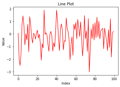
- Line plot
import pandas as pd
import numpy as np
import matplotlib.pyplot as plt

# Create a DataFrame with some random data
df = pd.DataFrame(np.random.randn(100, 4), columns=list('ABCD'))

# Plot a line chart of column A
df['A'].plot(kind='line', color='red', title='Line Plot')
plt.xlabel('Index')
plt.ylabel('Value')
plt.show()
This code creates a DataFrame with 100 rows and 4 columns of random data and then plots a line chart of column A using the “.plot” method. The “kind” parameter is set to “line” to create a line plot, and the “color” parameter is set to “red” to change the color of the line. The title, xlabel, and ylabel of the plot are also set using the standard Matplotlib functions.
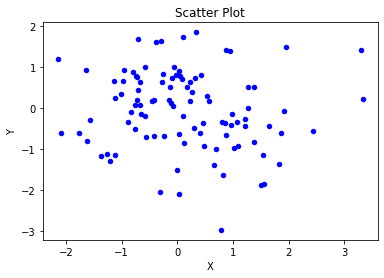
2. Scatter plot
import pandas as pd
import numpy as np
import matplotlib.pyplot as plt

# Create a DataFrame with some random data
df = pd.DataFrame(np.random.randn(100, 2), columns=['X', 'Y'])

# Plot a scatter chart of columns X and Y
df.plot(kind='scatter', x='X', y='Y', color='blue', title='Scatter Plot')
plt.xlabel('X')
plt.ylabel('Y')
plt.show()
This code creates a DataFrame with 100 rows and 2 columns of random data and then plots a scatter chart of columns X and Y using the “.plot” method. The “kind” parameter is set to “scatter” to create a scatter plot, and the “x” and “y” parameters are set to ‘X’ and ‘Y’ respectively to specify the columns to use as the x-axis and y-axis of the plot.
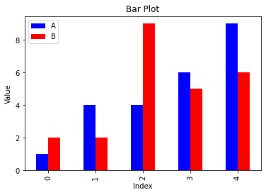
3. Bar plot
import pandas as pd
import numpy as np
import matplotlib.pyplot as plt

# Create a DataFrame with some random data
df = pd.DataFrame({'A': np.random.randint(1, 10, 5), 'B': np.random.randint(1, 10, 5)})

# Plot a bar chart of columns A and B
df.plot(kind='bar', color=['blue', 'red'], title='Bar Plot')
plt.xlabel('Index')
plt.ylabel('Value')
plt.show()
This code creates a DataFrame with 5 rows and 2 columns of random data and then plots a bar chart of columns A and B using the “.plot” method. The “kind” parameter is set to “bar” to create a bar plot, and the “color” parameter is set to a list of colors to use for the bars.
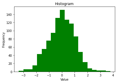
4. Histogram
import pandas as pd
import numpy as np
import matplotlib.pyplot as plt

# Create a DataFrame with some random data
df = pd.DataFrame(np.random.randn(1000, 1), columns=['A'])

# Plot a histogram of column A
df['A'].plot(kind='hist', bins=20, color='green', title='Histogram')
plt.xlabel('Value')
plt.show()
This code creates a DataFrame with 1000 rows and 1 column of random data and then plots a histogram of column A using the “.plot” method. The “kind” parameter is set to “hist” to create a histogram, and the “bins” parameter is set to 20 to control the number of bins in the histogram.
9. Aggregation Manually instead of using .groupby()
Aggregation is a common operation in data analysis where we group data based on one or more columns and apply a mathematical function to the remaining columns to get summarized information about the data. Pandas provide a .groupby() method that simplifies the process of aggregation, but manually performing aggregation can lead to inefficient code.
Here are some examples of manually aggregating data in Pandas and how it can be improved using .groupby():
- Manually aggregating by looping through each group:
import pandas as pd

df = pd.read_csv('sales_data.csv')

unique_regions = df['region'].unique()

for region in unique_regions:
    region_sales = df[df['region'] == region]['sales']
    total_sales = region_sales.sum()
    average_sales = region_sales.mean()
    max_sales = region_sales.max()
    min_sales = region_sales.min()
    print(f'{region}: Total Sales: {total_sales}, Average Sales: {average_sales}, Max Sales: {max_sales}, Min Sales: {min_sales}')
This code loops through each unique region in the dataset filters the data for that region and manually calculates the total, average, maximum, and minimum sales for that region. This process can be simplified using .groupby():
import pandas as pd

df = pd.read_csv('sales_data.csv')

region_stats = df.groupby('region')['sales'].agg(['sum', 'mean', 'max', 'min'])
print(region_stats)
This code groups the data by the region column and calculates the total, average, maximum, and minimum sales for each region using the .agg() method.
2. Manually aggregating by creating multiple pivot tables
import pandas as pd

df = pd.read_csv('sales_data.csv')

region_sales = pd.pivot_table(df, index='region', values='sales', aggfunc=['sum', 'mean', 'max', 'min'])
category_sales = pd.pivot_table(df, index='category', values='sales', aggfunc=['sum', 'mean', 'max', 'min'])
product_sales = pd.pivot_table(df, index='product', values='sales', aggfunc=['sum', 'mean', 'max', 'min'])

print(region_sales)
print(category_sales)
print(product_sales)
This code creates multiple pivot tables to calculate the total, average, maximum, and minimum sales for each region, category, and product. This can be simplified using .groupby():
import pandas as pd

df = pd.read_csv('sales_data.csv')

sales_stats = df.groupby(['region', 'category', 'product'])['sales'].agg(['sum', 'mean', 'max', 'min'])
print(sales_stats)
This code groups the data by the region, category, and product columns and calculates the total, average, maximum, and minimum sales for each combination of those columns using the .agg() method.
Overall, manually aggregating data can be time-consuming and error-prone, especially for large datasets. The .groupby() method simplifies the process and provides a more efficient and reliable way to perform aggregation operations in Pandas.
10. Saving Large Datasets as CSV File
While saving large datasets as CSV files is a common and simple approach, it may not always be the best option. Here are some reasons why:
- Large file size: CSV files can be very large in size, especially when dealing with datasets that have many columns and/or rows. This can cause problems with storage and processing, especially if you have limited resources.
- Limited data types: CSV files only support a limited range of data types, such as text, numbers, and dates. If your dataset includes more complex data types, such as images or JSON objects, then CSV may not be the best format to use.
- Loss of metadata: CSV files do not support metadata, such as data types, column names, or null values. This can cause problems when importing or exporting the data, and can make it difficult to perform data analysis.
- Performance issues: Reading and writing large CSV files can be slow and can put a strain on system resources, especially when dealing with complex datasets.
- No data validation: CSV files do not provide any built-in data validation or error checking, which can lead to data inconsistencies and errors.
There are more efficient ways to save large dataframes than using CSV files. Some of the options are:
- Parquet: Parquet is a columnar storage format that is optimized for data processing on large data sets. It can handle complex data types and supports compression, which makes it a good choice for storing large dataframes.
- Feather: Feather is a lightweight binary file format designed for fast read and write operations. It supports both R and Python and can be used to store dataframes in a compact and efficient way.
- HDF5: HDF5 is a file format designed for storing large numerical data sets. It provides a hierarchical structure that can be used to organize data and supports compression and chunking, which makes it suitable for storing large dataframes.
- Apache Arrow: Apache Arrow is a cross-language development platform for in-memory data processing. It provides a standardized format for representing data that can be used across different programming languages and supports zero-copy data sharing, which makes it efficient for storing and processing large dataframes.
Each of these options has its own strengths and weaknesses, so the choice of which one to use depends on your specific use case and requirements.
If you like the article and would like to support me make sure to:
- 👏 Clap for the story (50 claps) to help this article be featured
- Follow me on Medium
- 📰 View more content on my medium profile
- 🔔 Follow Me: LinkedIn |Youtube | GitHub | Twitter
Join the Medium membership program for only 5$ to continue learning without limits. I’ll receive a small portion of your membership fee if you use the following link, at no extra cost to you.
Looking to start a career in data science and AI and do not know how. I offer data science mentoring sessions and long-term career mentoring:
- Long-term mentoring: https://lnkd.in/dtdUYBrM
- Mentoring sessions: https://lnkd.in/dXeg3KPW