Matplotlib: Examples for Financial and Geographical Cases

Exploring the power of Matplotlib with some examples

The article shows two examples for financial and geographical applications. Matplotlib is commonly used for visualizing financial data, such as stock prices, exchange rates, and economic indicators, and provides a variety of chart types ideal for time series data, including line charts, bar charts, and scatter plots. The article provides an example of using Matplotlib to create a candlestick chart, which shows the opening, closing, high, and low prices of a security over a specific period of time, using the mpl_finance and yfinance libraries. The article also discusses how Matplotlib can be used for geographical data plotting, such as creating choropleth maps and scatter plots that represent data by shading or coloring different regions or areas. An example of creating a Europe map with all countries colored in green except for Spain, which is colored in blue, is provided using the Cartopy library. Cartopy is a powerful Python library that provides tools for creating maps and working with geospatial data.

Financial Data Plotting

Matplotlib is commonly used to plot financial data such as stock prices, exchange rates, and economic indicators. It provides a variety of chart types such as line charts, bar charts, and scatter plots, which are ideal for visualizing time series data.

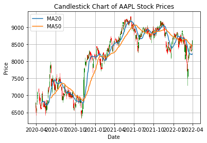
For example, you can use Matplotlib to create candlestick charts, which show the opening, closing, high, and low prices of a security over a specific period of time. Additionally to matplotlib, mpl_finance and yfinance libraries are used for this example.

The mpl_finance library is used in this example to create a candlestick chart, which is a type of financial chart used to represent the opening, closing, high, and low prices of a security over a specific period of time.

The yfinance library is used in this example to download the stock prices data directly from Yahoo Finance. This library provides a simple and convenient way to access financial data from Yahoo

import matplotlib.pyplot as plt
from mpl_finance import candlestick_ohlc
import yfinance as yf
import matplotlib.dates as mdates
import pandas as pd

# set stock symbol and start and end dates
symbol = '^IBEX'
start_date = '2020-03-30'
end_date = '2022-03-30'

# download stock prices data from Yahoo Finance
data = yf.download(symbol, start=start_date, end=end_date)

# reset index and convert date column to datetime object
data = data.reset_index()

# create moving averages
data['MA20'] = data['Close'].rolling(window=20).mean()
data['MA50'] = data['Close'].rolling(window=50).mean()

# create figure and axis objects
fig, ax = plt.subplots()

# format x-axis as dates
ax.xaxis_date()

# set labels and title
ax.set_xlabel('Date')
ax.set_ylabel('Price')
ax.set_title('Candlestick Chart of AAPL Stock Prices')

# create candlestick chart
ohlc = data[['Date', 'Open', 'High', 'Low', 'Close']].copy()
ohlc['Date'] = ohlc['Date'].apply(mdates.date2num)
candlestick_ohlc(ax, ohlc.values, width=0.6, colorup='green', colordown='red')

# plot moving averages
ax.plot(data['Date'], data['MA20'], label='MA20')
ax.plot(data['Date'], data['MA50'], label='MA50')

# add legend
ax.legend()

# show plot
plt.show()

In this modified example, the yfinance library is used to download the stock prices data by passing in the stock symbol, start and end dates to the download function. In the example, IBEX 35 data from 2020 to the end of 2021 has been downloaded. The downloaded data is then reset the index as before. The ohlc DataFrame is created to extract the OHLC values and convert the date column to a numerical format that can be used with the candlestick_ohlc function. Finally, Moving Averate (MA) with windows of 20 and 50 are also computed and plotted.

Geographical Data Plotting

Geographical data plotting is an essential task for many applications, such as climate studies, population analysis, and resource management. Matplotlib is a powerful Python library that provides various map projections and geographic coordinate systems to choose from, making it ideal for displaying data associated with a specific location. With Matplotlib, you can create choropleth maps, scatter plots, and other visualizations that represent data by shading or coloring different regions or areas. In this way, you can gain insights into spatial patterns and relationships that are not easily visible in tabular data. In the following sections, we will explore some examples of how Matplotlib can be used for geographical data plotting.

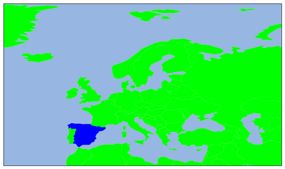
Below, an example of geographical data plotting using Matplotlib is showed. The code plots a Europe map with all countries colored in green appart from Spain, which is colored in blue. To do so, cartopy library is also used. Cartopy is a Python library that provides powerful tools for creating maps and working with geospatial data. It is built on top of the matplotlib library and integrates seamlessly with its data visualization capabilities. Cartopy supports a wide range of map projections and coordinate systems, allowing you to create maps that are tailored to your specific needs. In addition, Cartopy provides built-in support for accessing and working with data from popular geospatial data sources, such as Natural Earth and NASA.

import matplotlib.pyplot as plt
import cartopy
import cartopy.io.shapereader as shpreader
import cartopy.crs as ccrs

ax = plt.axes(projection=ccrs.PlateCarree())
#ax.add_feature(cartopy.feature.LAND)
ax.add_feature(cartopy.feature.OCEAN)
#ax.add_feature(cartopy.feature.COASTLINE)
#ax.add_feature(cartopy.feature.BORDERS, linestyle='-', alpha=.5)
#ax.add_feature(cartopy.feature.LAKES, alpha=0.95)
#ax.add_feature(cartopy.feature.RIVERS)
ax.set_extent([-150, 60, -25, 60])

shpfilename = shpreader.natural_earth(resolution='110m',
                                      category='cultural',
                                      name='admin_0_countries')
reader = shpreader.Reader(shpfilename)
countries = reader.records()


for country in countries:
    if country.attributes['NAME_EN'] == 'Spain':
        print("Spain")
        ax.add_geometries(country.geometry, ccrs.PlateCarree(),
                          facecolor=(0, 0, 1),
                          label=country.attributes['NAME_EN'])
    else:
        print("Spain")
        ax.add_geometries(country.geometry, ccrs.PlateCarree(),
                          facecolor=(0, 1, 0),
                          label=country.attributes['NAME_EN'])

plt.show()

This code uses the Cartopy library to create a choropleth map of the Europ with countries colored based on a condition. First, the code imports the necessary libraries and defines a Plate Carree projection. Then, it sets the extent of the map to be displayed.

The code reads the shapefile of the countries from the Natural Earth dataset and creates a Reader object. It then iterates through the countries and checks if the country name is Spain. If it is, the code adds the country’s geometry to the map with a blue color. Otherwise, it adds the country’s geometry with a green color.

Finally, the code displays the map using the plt.show() function. The commented-out lines of code show how to add other features to the map, such as land, coastlines, and borders. By default, the map displays only the ocean feature.

Course index:

Have you spent your learning budget for this month, you can join Medium here:

Level Up Coding

Thanks for being a part of our community! Before you go:

• 👏 Clap for the story and follow the author 👉
• 📰 View more content in the Level Up Coding publication
• 💰 Free coding interview course ⇒ View Course
• 🔔 Follow us: Twitter | LinkedIn | Newsletter

🚀👉 Join the Level Up talent collective and find an amazing job