Mathematical Guide to Modelling the Distribution of Asset Returns
I will be introducing how to model the distribution of the S&P500 returns. I will be exploring the parameterized models normal, student-t, skewed normal and also non-parameteized models; KDE and TKDE.

Introduction
Being able to successfully model the distribution of asset returns is a important part of quantitative finance. The distribution of asset returns is used in many applications. Two examples would be option pricing and portfolio management. In portfolio management we look to understand the expected return and variance of the portfolio. Additionally with new research in deep learning we may need to simulate the market and require statistical methods that require a model for the asset returns.
The aim is to mathematically model the distribution of the ETF ‘SPY’
Back before 1998 it was understood that asset returns are normally distributed, now we know that heavy tails represent highly volatile days and need to be considered in the model. In this article, I look to explore the student-t and skewed distributions and compare back to the normal distribution.
Parametrized Statistical Models
Parametrized models are statistical models in which all its information is represented within it's parameters. The information in our case is the asset returns and the parameters would be mu and sigma in the normal distribution.
The underlying assumption is the returns follow a normal distribution, what this means is using mu and sigma we are able to model the data using a normal distribution structure. Any distribution can be used to model the asset return, we begin with the normal distribution.
For the parametrized normal distribution the mean and standard deviation are found using the maximum likelihood method from the data.
By using the Normal PDF our assumption is the data follows the normal distribution curve.
In other words the distribution of the data is completely specified except for a finite number of unknown parameters.
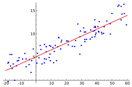
I quickly introduce the linear regression model to highlight how the parameters are fit to a dataset. Again the assumption is the relationship is linear and our goal is to find the numerical values for the slope and Y-intercept.
Below is an example of a linear regression model fit using MSE. Understand that the distance from each blue point to the line is measured then squared and finally divided by the total number of data points.
The formula for the mean squared error (MSE) is given as
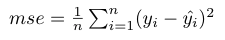
From the MSE formula the hat represents the predicted or estimated values for the variable y. In mathematics the hat above the variable represents an estimation for a given random variable. n represents the number of total data points that we our estimating. The graphic above shows how the MSE would be calculated for a simple linear regression model in two dimensions.
Non-Parametrized Statistical models
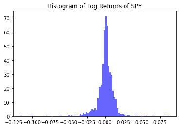
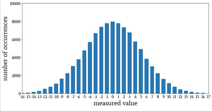
In statistics a non-parametrized model is one where this is no fixed or a priori distribution or model structure. The most basic would be a histogram where we sort the data into buckets representing its numerical value.
Moving past the histogram I introduce the kernel density estimator (KDE). Often a kernel density estimate is used to suggest a parametric statistical model. The KDE formula is given as
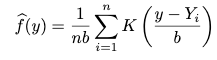
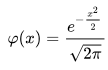
K, which is a probability density function that is symmetric about 0. b, which is called the bandwidth, determines the resolution of the estimator. A typical choice for K is the standard normal distribution. A standard normal is when mu = 0 and sigma =1.
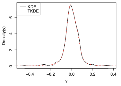
Extending the KDE to the transformed kernel density estimation (TKDE). A better density estimate can be obtained by the transformation kernel density estimator (TKDE). The idea is to transform the data so that the density of the transformed data is easier to estimate by the KDE.
The transformation to use in the TKDE is g(y) = Φ−1{F(y)}, which has inverse g−1(x) = F−1{Φ(x)}. Phi is the CDF of the normal distribution.
Kernel Density Estimator
Implementing the KDE in python on one dimensional data.
kde = KernelDensity(kernel="gaussian",bandwidth=0.3).fit(data.reshape(-1,1))The bandwidth is selected automatically using the log-likelihood. If you get higher likelihoods for a bandwidth value, the data is represented with that given bandwidth the best.
A small bandwidth leads to a high-variance estimate, where the presence or absence of a single point makes a large difference. Too large a bandwidth leads to a high-bias estimate where the structure in the data is washed out by the wide kernel.
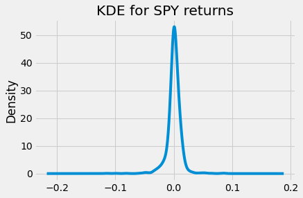
From the KDE the density of the returns are concentrated around a mean of zero.
Maximum Likelihood Estimation
Maximum likelihood is the main method of estimating parameters for different mathematical models. As an example, for a normal distribution, the maximum likelihood estimator of the mean is more efficient than the sample mean.
Let Y = (Y1,…,Yn) be a vector of data and let θ = (θ1,…,θp) be a vector of parameters. Let f(Y |θ) be the density of Y , which depends on the parameters.
The function L(θ) = f(Y |θ) viewed as a function of θ with Y fixed at the observed data is called the likelihood function. It tells us the likelihood of the sample that was actually observed. The maximum likelihood estimator (MLE) is the value of θ that maximizes the likelihood function. In other words, maximum likelihood estimation (MLE) finds the value of θ at which the likelihood of the observed data is largest.
In practice when using computer software we end up finding the minimum or the min(−L(θ)).
The likelihood function for the normal distribution is given as
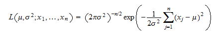
The likelihood function represents the probability of mu & sigma in a normal distribution structure given data; Xn. Using some simple calculus principles we know we need to take the derivative of the likelihood and set it equal to zero to find the maximum of the function.
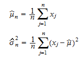
Rearranging for mu & sigma we find the parameter estimation for the Gaussian model using the maximum likelihood estimation.
Normal Distribution
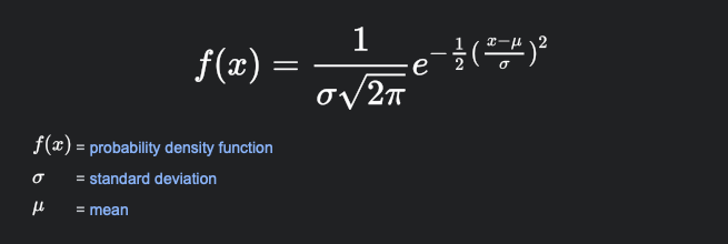
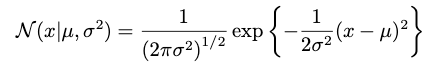
The normal Distribution is a probability function where the area under the curve in one dimension sums to 1. The X interval is between (-inf,+inf).
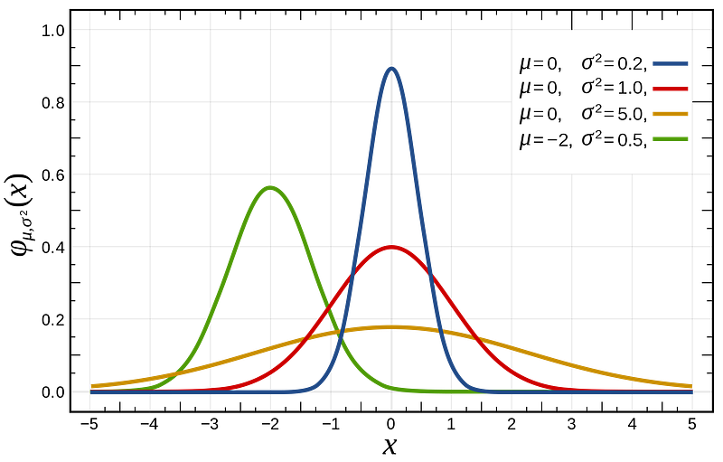
For any of the given normal distributions the sum of the area under the curve is equal to 1. Intuitively this makes sense, if we were to sum all the probabilities we would get one. We can’t have a probability that is greater than 100%.
The formula for the univariable normal distribution is given as
Modelling the S&P500 returns using a normal distribution
Using Python, I want to fit the log(Price(t+1)-log(Price(t))/log(Price(t+1)) using a normal distribution. The purpose of using the log of the price is to de-trend the data and produce a stationary time series.
import yfinance as yf  #import data via Yahoo
today = datetime.today()
sp_list = ['SPY']
offset = max(1, (today.weekday() + 6) % 7 - 3)
timed = timedelta(offset)
today_business = today - timed
print("d1 =", today_business)
today = today_business.strftime("%Y-%m-%d")
start = '2017-01-01'
end = today
print('S&P500 Stock download')
spy = yf.download(sp_list, start,end)
from scipy.stats import norm
# Generate some data for this demonstration.
log_return = (np.diff(np.log(spy.Close),axis=0))
spy = spy.iloc[1:,:]
spy['log_return'] = log_return
data = spy.log_return.values
# Fit a normal distribution to the log daily returns:
mu, std = norm.fit(data)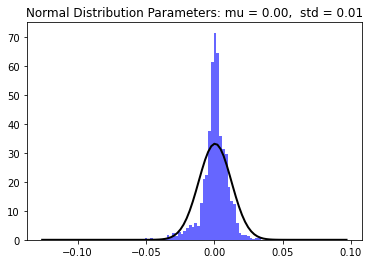
The normal distribution is represented with the black line with, mu = 0.00058549 and sigma = 0.012014. Here our mean is positive which makes sense since market returns are generally positive over time.
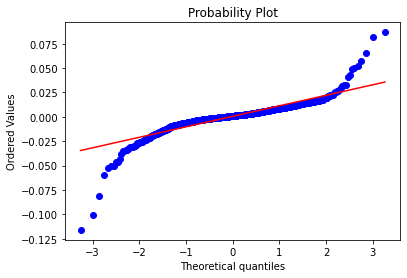
A probability plot of sample data against the quantiles of a normal distribution was generated for interpretation. Here it is clear that the normal distribution is not representative of the log returns of ‘SPY’. The normal distribution does a good job of fitting middle section of the data, however the tails differ significantly.
Observing the tails of the distribution, the normal distribution does a poor job of capturing daily returns that deviate significantly from the average. The mean and the skewness is also not captured.
Let us ponder if our mean was equal to 0 meaning that over time the market had a expected return of 0. Say we were to deploy a trading Algorithm that takes a long or short position, regardless of our strategy the expected return given a extremely long period of time is zero. This is something to keep in mind when trading various financial markets, before exhausting time and resources creating a strategy, checking the expected return of the financial market you are looking to trade is a good place to start.
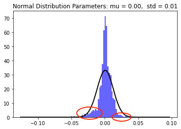
Let us zoom in and pay particular to the two red circles representing the tails of the log returns of ‘SPY’. The left tail has a higher density then the right tail to address this we will need to model the skewness of the data.
Student-T Distribution
More recently, t-distributions have gained added importance as models for the distribution of heavy-tailed phenomena such as financial markets data. The student-t distribution takes three parameters as input (DoF, mu,std). The degrees of freedom are a value that alters the tails and peak of the distribution. When DoF approaches infinity the student-t distribution simply becomes the normal distribution. The PDF of the student-t distribution is given as
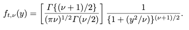
The Student-t (T) distribution is a probability function where the area under the curve in two dimensions sums to 1. The X interval is between (-inf,+inf).
The DoF is a third parameter of the T-distribution which models the tails of the distribution. See how by varying the DoF and holding mu & sigma constant that heavy tails can be modelled. It is for this reason that the student-t distribution is now common use in the industry for understanding asset returns.
Modelling the S&P500 returns using a student-t distribution
Moving onwards to the student-t distribution modelling in python.
from scipy.stats import t
# Fit a normal distribution to the data:
dof, mu, std = t.fit(data)
xmin, xmax = plt.xlim([-0.1,0.1])
x = np.linspace(xmin, xmax, 1000)
p1 = t.pdf(x,dof, mu, std)
plt.hist(data, bins=100, density=True, alpha=0.6, color='b')
# Plot the PDF.
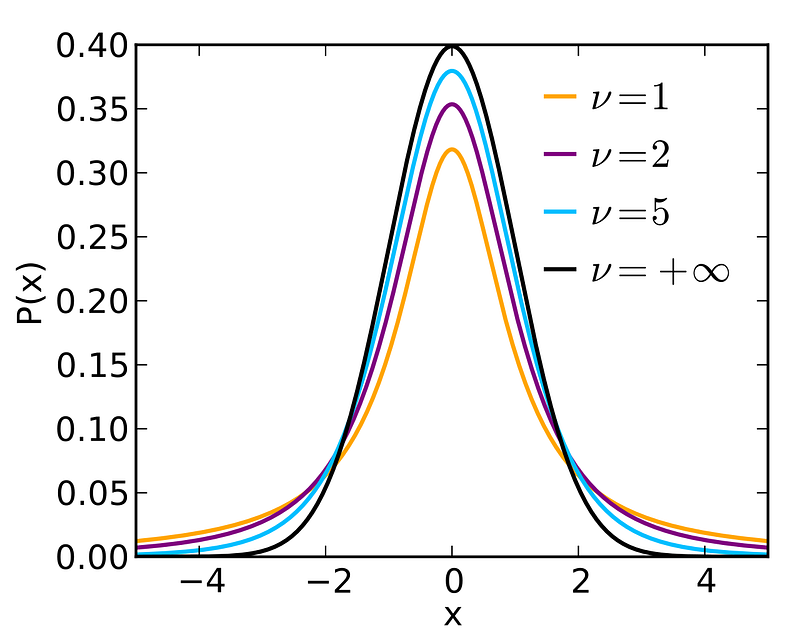
plt.plot(x, p1, 'k' ,linewidth=2,label='SPY Log Returns')
title = "Student-t Distribution SPY Fitting"
plt.title(title)
plt.legend()
plt.show()The student-t distribution is a much better model for fitting the log returns of a financial asset compared to the normal distribution.
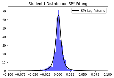
To understand how well the distribution model is fit to the data I produce the Q-Q plot.
The student-t distribution does a much better job of fitting the data, however the skewness of the tails are not captured. From the probability plot the left tail is being under fit and the right tail is being overfit. The student-t distribution does a much better job of modelling the data however I will continue to approve upon this model.
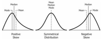
Skewed Distributions
A skewed distribution is occurs when the mean and medium take on different values.
A very good example of positive skewed data is component time to failure, this is a case where some components may last extremely long while others may experience early failure (sometimes this is called a lemon). The Weibull distribution does a very good job of modelling component time to failure.
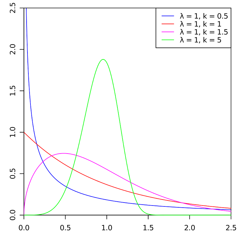
The pink line is typical of component time to failure probability.
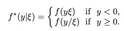
Fernandez and Steel have devised a clever way for inducing skewness in symmetric distributions such as normal and t-distributions.
If ξ > 1, then the right half of f(y|ξ) is elongated relative to the left half, which induces right skewness. Similarly, ξ < 1 induces left skewness.
Let ξ be a positive constant and f a density that is symmetric about 0
Skewed Normal Distribution
The skewed normal distribution was first introduced to capture non-zero skewness.
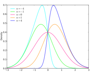
The formula for the skewd normal distribution is given as
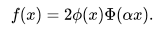
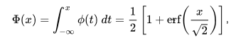
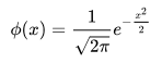
Here lower-case Phi is the probability density function for the normal distribution and upper-case Phi is the cumulative distribution function.
Fitting the normal skewed distribution in python is done in the following way.
from scipy.stats import skewnorma, loc, scale = skewnorm.fit(data)
skewnorm.pdf(x, a, loc, scale)The additional parameter used to model the skewness is (a). Simliar to both the normal and student-t distribution the skewed normal is fit using the MLE method.
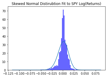
If you look closer the normal distribution will appear skewed to the left capturing part of the density towards the left of the histogram.
Conclusion
Everything that was shown in this article was done to apply statistical distributions using real data. To improve the robustness of modelling the returns of financial markets different distributions were tested and the results shown.
About the author:
Ethan Skinner holds a Master’s of Applied Mathematics from Ryerson University, in Toronto, Canada, where he also completed his Bachelor’s in Aerospace Engineering. Ethan has published two academic papers at the IEEE COMSAC 2021 conference.
He was part of the financial mathematics group specializing in statistics, and studied volatility modelling and algorithmic trading in-depth. Ethan previously worked as an engineering professional at Bombardier Aerospace, where he was responsible for modelling the life-cycle costs associated with aircraft maintenance.
I am actively training for triathlon and love fitness.
If you have any suggestions on the topics below let me know
- Data science
- Machine Learning
- Mathematics
- Statistical Modelling
LinkedIn: https://www.linkedin.com/in/ethanjohnsonskinner/
Twitter : @Ethan_JS94


