Mastering Long Short-Term Memory with Python: Unleashing the Power of LSTM in NLP

A comprehensive guide to understanding and implementing LSTM layers for natural language processing with Python

This work is a continuation of my article about RNNs and NLP with Python. A natural progression of a deep learning network with a simple recurrent layer is a deep learning network with a Long Short Term Memory (LSTM for short) layer.

As with the RNN and NLP, I will try to explain the LSTM layer in great detail and code the forward pass of the layer from scratch.

All the codes can be viewed here: https://github.com/Eligijus112/NLP-python

We will work with the same dataset¹ as in the previous article:

# Data wrangling
import pandas as pd

# Reading the data 
d = pd.read_csv('input/Tweets.csv', header=None)

# Adding the columns 
d.columns = ['INDEX', 'GAME', "SENTIMENT", 'TEXT']

# Leaving only the positive and the negative sentiments 
d = d[d['SENTIMENT'].isin(['Positive', 'Negative'])]

# Encoding the sentiments that the negative will be 1 and the positive 0
d['SENTIMENT'] = d['SENTIMENT'].apply(lambda x: 0 if x == 'Positive' else 1)

# Dropping missing values
d = d.dropna()

Random rows from the dataset; Picture by author

Remember, that SENTIMENT=1 is a negative sentiment, and SENTIMENT=0 is a positive sentiment.

We need to convert the text data into a sequence of integers. Unlike in the previous article though, we will now create a sequence not of words but of individual characters.

For example, the text “Nice Game” could be converted to the following example vector:

[1, 2, 3, 4, 5, 6, 7, 8, 3]

Each individual character, including whitespaces and punctuations, will have an index.

def create_word_index(
    x: str, 
    shift_for_padding: bool = False, 
    char_level: bool = False) -> Tuple[dict, dict]: 
    """
    Function that scans a given text and creates two dictionaries:
    - word2idx: dictionary mapping words to integers
    - idx2word: dictionary mapping integers to words

    Args:
        x (str): text to scan
        shift_for_padding (bool, optional): If True, the function will add 1 to all the indexes.
            This is done to reserve the 0 index for padding. Defaults to False.
        char_level (bool, optional): If True, the function will create a character level dictionary.
        
    Returns:
        Tuple[dict, dict]: word2idx and idx2word dictionaries
    """
    # Ensuring that the text is a string
    if not isinstance(x, str):
        try: 
            x = str(x)
        except:
            raise Exception('The text must be a string or a string convertible object')
        
    # Spliting the text into words
    words = []
    if char_level:
        # The list() function of a string will return a list of characters
        words = list(x)
    else:
        # Spliting the text into words by spaces
        words = x.split(' ')

    # Creating the word2idx dictionary 
    word2idx = {}
    for word in words: 
        if word not in word2idx: 
            # The len(word2idx) will always ensure that the 
            # new index is 1 + the length of the dictionary so far
            word2idx[word] = len(word2idx)

    # Adding the <UNK> token to the dictionary; This token will be used 
    # on new texts that were not seen during training.
    # It will have the last index. 
    word2idx['<UNK>'] = len(word2idx)

    if shift_for_padding:
        # Adding 1 to all the indexes; 
        # The 0 index will be reserved for padding
        word2idx = {k: v + 1 for k, v in word2idx.items()}

    # Reversing the above dictionary and creating the idx2word dictionary
    idx2word = {idx: word for word, idx in word2idx.items()}

    # Returns the dictionaries
    return word2idx, idx2word

Let us split our data into a train-test split and apply our created function:

# Spliting to train test 
train, test = train_test_split(d, test_size=0.2, random_state=42)

# Reseting the indexes 
train.reset_index(drop=True, inplace=True)
test.reset_index(drop=True, inplace=True)

print(f'Train shape: {train.shape}')
print(f'Test shape: {test.shape}')
Train shape: (34410, 4)
Test shape: (8603, 4)

# Joining all the texts into one string
text = ' '.join(train['TEXT'].values)

# Creating the word2idx and idx2word dictionaries
word2idx, idx2word = create_word_index(text, shift_for_padding=True, char_level=True)

# Printing the size of the vocabulary
print(f'The size of the vocabulary is: {len(word2idx)}')
The size of the vocabulary is: 274

There are 274 unique characters in our data. Let us print the top 10 entries in our word2idx dictionary:

{'I': 1,
 ' ': 2,
 'd': 3,
 'o': 4,
 'w': 5,
 'n': 6,
 'l': 7,
 'a': 8,
 'e': 9,
 'G': 10
}

Let us convert the texts to sequences:

# For each row in the train and test set, we will create a list of integers
# that will represent the words in the text
train['text_int'] = train['TEXT'].apply(lambda x: [word2idx.get(word, word2idx['<UNK>']) for word in list(x)])
test['text_int'] = test['TEXT'].apply(lambda x: [word2idx.get(word, word2idx['<UNK>']) for word in list(x)])

# Calculating the length of sequences in the train set 
train['seq_len'] = train['text_int'].apply(lambda x: len(x))

# Describing the length of the sequences
train['seq_len'].describe()
count    34410.000000
mean       103.600262
std         79.972798
min          1.000000
25%         41.000000
50%         83.000000
75%        148.000000
max        727.000000

To recall, splitting the texts by word level led to the mean length of a sequence being equal to ~22 tokens. Now, we have sequences of length ~103 tokens. The standard deviation is very high, thus we will use the max sequence length of 200 in padding.

def pad_sequences(x: list, pad_length: int) -> list:
    """
    Function that pads a given list of integers to a given length

    Args:
        x (list): list of integers to pad
        pad_length (int): length to pad

    Returns:
        list: padded list of integers
    """
    # Getting the length of the list
    len_x = len(x)

    # Checking if the length of the list is less than the pad_length
    if len_x < pad_length: 
        # Padding the list with 0s
        x = x + [0] * (pad_length - len_x)
    else: 
        # Truncating the list to the desired length
        x = x[:pad_length]

    # Returning the padded list
    return x

# Padding the train and test sequences 
train['text_int'] = train['text_int'].apply(lambda x: pad_sequences(x, 200))
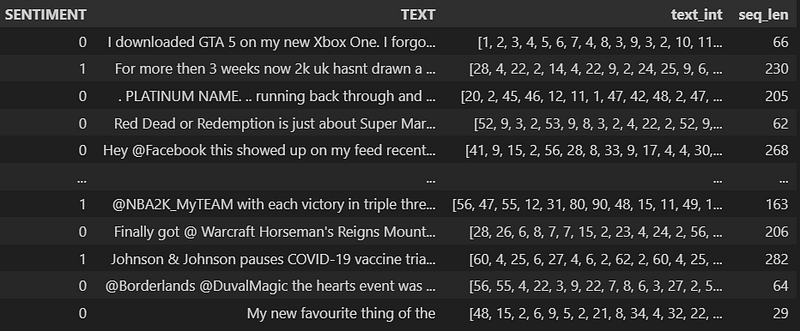
test['text_int'] = test['text_int'].apply(lambda x: pad_sequences(x, 200))

The train and val datasets thus far look like the following:

Why should we switch from a vanilla RNN to an LSTM network? The problems are twofold:

A simple RNN has the so-called vanishing gradient problem² or the exploding gradient problem associated with the weights used in the for loop of the network.
The network tends to “forget” the initial steps input of a long sequence of data.

To illustrate the forgetness, consider the example:

In our data, on average, there are 103 timesteps (the number of tokens in a text going from left to right). Recall the graph from the RNN article:

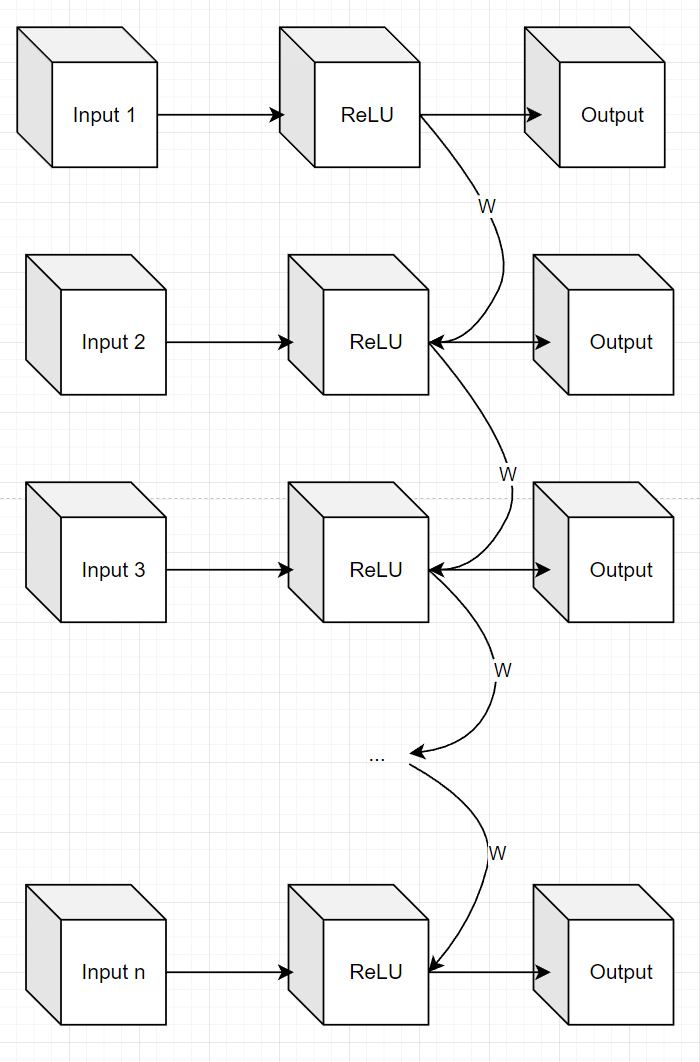
We have the same weight W that we multiply the output of the ReLU layer with. Then, we add that signal to the next time step, and so on. If we choose a relatively small value for W (let us say 0.5) and we have 103 steps of time series data, the impact from the first timestep input to the final output would be, roughly speaking, 0.5¹⁰³ * input1 which is approximately zero.

The signal from the second input would be 0.5¹⁰² * input2 and so on.

One can see, that the more timesteps we add, the less information is left to the final output from the initial time steps.

To battle this problem of forgetting the past, great minds have come up with an LSTM layer³ for use in time series problems.

Internally, an LSTM layer uses two activation functions:

Sigmoid function
Tanh function

Key facts to remember about these functions are:

The sigmoid activation function takes in any value on a real number plane and outputs a value between 0 and 1.
The tanh function takes in any value on a real number plane and outputs a value between -1 and 1.

def sigmoid(x: float) -> float: 
    """
    Function that calculates the sigmoid of a given value

    Args:
        x (float): value to calculate the sigmoid

    Returns:
        float: sigmoid of the given value in (0, 1)
    """
    return 1 / (1 + np.exp(-x))

def tanh(x: float) -> float: 
    """
    Function that calculates the tanh of a given value

    Args:
        x (float): value to calculate the tanh

    Returns:
        float: tanh of the given value in (-1, 1)
    """
    return (np.exp(x) - np.exp(-x)) / (np.exp(x) + np.exp(-x))

Now that we have the sigmoid and tanh activation functions in our minds, let us return to the LSTM layer. The LSTM layer is made up of 2 parts (hence the name):

Long-term memory block
Short-term memory block

At every time step (or token step), the LSTM layer outputs two predictions, the long-term prediction and the short-term prediction. A high-level diagram of an LSTM unit can be visualized like this:

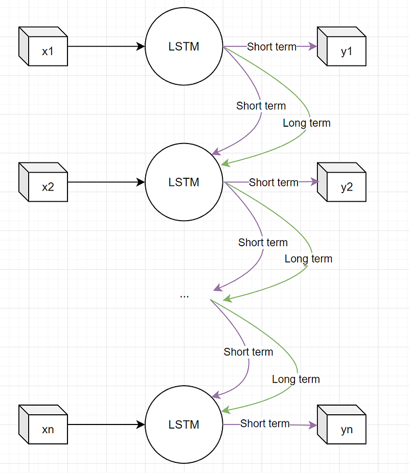
Unrolled simple LSTM network; Graph by author

At each time step, the LSTM layer outputs a number and this is what we call the short-term memory output. It is usually just a scalar. Additionally, the long-term memory scalar is also calculated in the LSTM layer but it is not output and transferred to the second step in the sequence. It is very important to note that at each time step, both the short-term and the long-term memories are updated.

Now let us dive deep into the LSTM layer. The first part of an LSTM layer is the so-called Forget Gate operation:

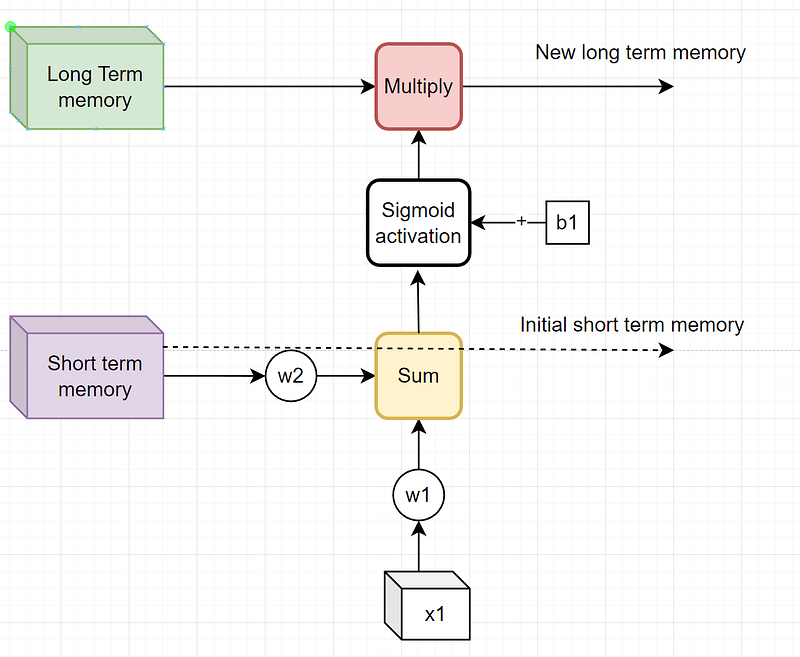
The forget gate gets its name from the fact that we calculate the percentage of the long-term memory that we want to keep. This is due to the fact that the sigmoid activation function will output a number between 0 and 1 and we will multiply that number by the long-term memory and pass it along the network.

We can start to see the weights that will be updated at training time: w1, w2, and b1. These weights directly influence the amount of long-term memory to keep.

Note that at this step, the short-term memory is not adjusted and gets passed along to the second steps of the network.

class ForgetGate: 
    """
    Class that implements the forget gate of an LSTM cell
    """
    def __init__(
            self, 
            w1: float = np.random.normal(), 
            w2: float = np.random.normal(),
            b1: float = np.random.normal(),
            long_term_memory: float = np.random.normal(), 
            short_term_memory: float = np.random.normal(), 
            ):
        """
        Constructor of the class

        Args:
            long_term_memory (float): long term memory
            short_term_memory (float): short term memory
            w1 (float): weight 1
            w2 (float): weight 2
            b1 (float): bias term 1
        """
        # Saving the input
        self.long_term_memory = long_term_memory
        self.short_term_memory = short_term_memory
        self.w1 = w1
        self.w2 = w2
        self.b1 = b1

    def forward(self, x: float) -> float: 
        """
        Function that calculates the output of the forget gate

        Args:
            x (float): input to the forget gate

        Returns:
            float: output of the forget gate
        """
        # Calculates the percentage of the long term memory that will be kept
        percentage_to_keep = sigmoid((self.w1 * x  + self.w2 * self.short_term_memory) + self.b1)

        # Updating the long term memory
        self.long_term_memory = self.long_term_memory * percentage_to_keep

        # The output of the forget gate is the new long term memory and the short term memory
        return self.long_term_memory, self.short_term_memory

# Initiating 
forget_gate = ForgetGate()

print(f'Initial long term memory: {forget_gate.long_term_memory}')
print(f'Initial short term memory: {forget_gate.short_term_memory}')

# Calculating the output of the forget gate
lt, st = forget_gate.forward(0.5)

print(f'Long term memory: {lt}')
print(f'Short term memory: {st}')

Initial long term memory: -0.8221542907288696
Initial short term memory: -0.5617438418718841
Long term memory: -0.37335827895028
Short term memory: -0.5617438418718841

Next up in the LSTM layer is the input gate:

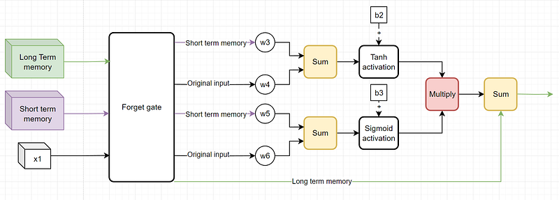
The input gate only adjusts the long-term memory part of the LSTM network, but in order to do that, it uses the current input and the current short-term memory values.

Looking at the graph, just before the multiplication step, we have two outputs: one from the sigmoid activation function and another from the tanh activation layer. Loosely speaking, the sigmoid layer outputs the percentage of the memory to remember (0, 1) and the tanh outputs the potential memory to remember (-1, 1).

We then sum up the current long-term memory, which was a bit adjusted in the forget gate, with the input gate output.

class InputGate:
    def __init__(
            self, 
            w3: float = np.random.normal(), 
            w4: float = np.random.normal(),
            w5: float = np.random.normal(),
            w6: float = np.random.normal(),
            b2: float = np.random.normal(),
            b3: float = np.random.normal(),
            long_term_memory: float = np.random.normal(), 
            short_term_memory: float = np.random.normal(), 
            ):
        """
        Constructor of the class

        Args:
            long_term_memory (float): long term memory
            short_term_memory (float): short term memory
            w3 (float): weight 3
            w4 (float): weight 4
            w5 (float): weight 5
            w6 (float): weight 6
            b2 (float): bias 2
            b3 (float): bias 3
        """
        # Saving the input
        self.long_term_memory = long_term_memory
        self.short_term_memory = short_term_memory
        self.w3 = w3
        self.w4 = w4
        self.w5 = w5
        self.w6 = w6
        self.b2 = b2
        self.b3 = b3

    def forward(self, x: float) -> float:
        """
        Function that calculates the output of the input gate

        Args:
            x (float): input to the input gate

        Returns:
            float: output of the input gate
        """
        # Calculating the memory signal 
        memory_signal = tanh((self.w3 * x + self.w4 * self.short_term_memory) + self.b2)

        # Calculating the percentage of memory to keep 
        percentage_to_keep = sigmoid((self.w5 * x + self.w6 * self.short_term_memory) + self.b3) 

        # Multiplying the memory signal by the percentage to keep
        memory_signal = memory_signal * percentage_to_keep

        # Updating the long term memory
        self.long_term_memory = self.long_term_memory + memory_signal

        # The output of the input gate is the new long term memory and the short term memory
        return self.long_term_memory, self.short_term_memory

# Creating the input gate object with the forget gates' output 
input_gate = InputGate(long_term_memory=lt, short_term_memory=st)

# Forward propagating 
lt, st = input_gate.forward(0.5)

print(f'Long term memory: {lt}')
print(f'Short term memory: {st}')

Long term memory: -1.028998511766425
Short term memory: -0.5617438418718841

As we can see from the code snippet above, the only thing that has changed is the long-term memory.

The last piece of the LSTM layer is the output gate. The output gate is the step where we will adjust the short-term memory of the layer:

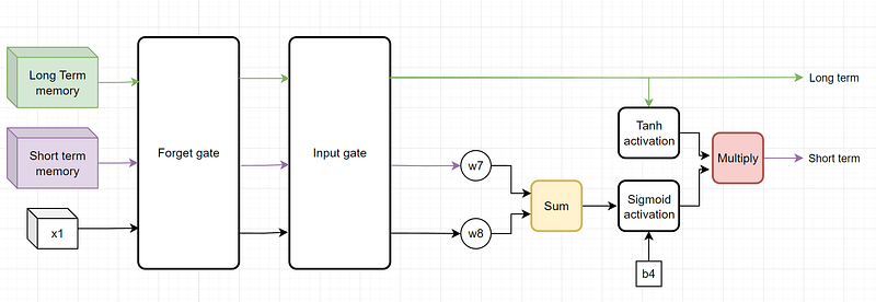
The logic is very similar to the logic that was present in the previous gates: the sigmoid activation calculates the percentage of memory to keep and the tanh function calculates the overall signal.

class OutputGate:
    def __init__(
            self, 
            w7: float = np.random.normal(), 
            w8: float = np.random.normal(),
            b4: float = np.random.normal(),
            long_term_memory: float = np.random.normal(), 
            short_term_memory: float = np.random.normal(), 
            ):
        """
        Constructor of the class

        Args:
            long_term_memory (float): long term memory
            short_term_memory (float): short term memory
            w7 (float): weight 7
            w8 (float): weight 8
            w9 (float): weight 9
            w10 (float): weight 10
            b4 (float): bias 4
            b5 (float): bias 5
        """
        # Saving the input
        self.long_term_memory = long_term_memory
        self.short_term_memory = short_term_memory
        self.w7 = w7
        self.w8 = w8
        self.b4 = b4

    def forward(self, x: float) -> float:
        """
        Function that calculates the output of the output gate

        Args:
            x (float): input to the output gate

        Returns:
            float: output of the output gate
        """
        # Calculating the short term memory signal 
        short_term_memory_signal = tanh(self.long_term_memory)

        # Calculating the percentage of short term memory to keep 
        percentage_to_keep = sigmoid((self.w7 * x + self.w8 * self.short_term_memory) + self.b4) 

        # Multiplying the short term memory signal by the percentage to keep
        short_term_memory_signal = short_term_memory_signal * percentage_to_keep

        # Updating the short term memory
        self.short_term_memory = short_term_memory_signal

        # The output of the output gate is the new long term memory and the short term memory
        return self.long_term_memory, self.short_term_memory

# Creating the output gate object
output_gate = OutputGate(long_term_memory=lt, short_term_memory=st)

# Forward propagating
lt, st = output_gate.forward(0.5)

print(f'Long term memory: {lt}')
print(f'Short term memory: {st}')

Long term memory: -1.028998511766425
Short term memory: -0.7233077589896045

As we can see, the output gate only adjusted the short-term memory scalar.

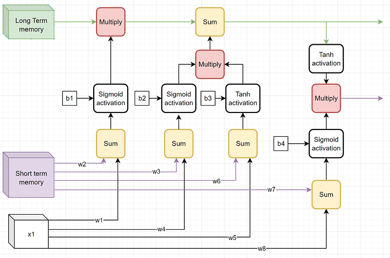
The above graph shows the forget, input, and output gates on one graph⁴.

When we have an input sequence of x variables, the inner loop when using the LSTM layer is this:

Initiate randomly short-term and long-term memory.

2. For each x1 to xn:

2.1 Forward propagate through the LSTM layer.

2.2 Output the short-term memory

2.3 Save the long-term and short-term memories to the layer.

Let us wrap every gate to a class and create a Python example.

# Redefining the forget, input and output gates as functions 
def forget_gate(x: float, w1: float, w2: float, b1: float, long_term_memory: float, short_term_memory: float) -> Tuple[float, float]:
    """
    Function that calculates the output of the forget gate

    Args:
        x (float): input to the forget gate
        w1 (float): weight 1
        w2 (float): weight 2
        b1 (float): bias 1
        long_term_memory (float): long term memory
        short_term_memory (float): short term memory

    Returns:
        Tuple[float, float]: output of the forget gate
    """
    # Calculates the percentage of the long term memory that will be kept
    percentage_to_keep = sigmoid((w1 * x  + w2 * short_term_memory) + b1)

    # Updating the long term memory
    long_term_memory = long_term_memory * percentage_to_keep

    # The output of the forget gate is the new long term memory and the short term memory
    return long_term_memory, short_term_memory

def input_gate(x: float, w3: float, w4: float, w5: float, w6: float, b2: float, b3: float, long_term_memory: float, short_term_memory: float) -> Tuple[float, float]:
    """
    Function that calculates the output of the input gate

    Args:
        x (float): input to the input gate
        w3 (float): weight 3
        w4 (float): weight 4
        w5 (float): weight 5
        w6 (float): weight 6
        b2 (float): bias 2
        b3 (float): bias 3
        long_term_memory (float): long term memory
        short_term_memory (float): short term memory

    Returns:
        Tuple[float, float]: output of the input gate
    """
    # Calculating the memory signal 
    memory_signal = tanh((w3 * x + w4 * short_term_memory) + b2)

    # Calculating the percentage of memory to keep 
    percentage_to_keep = sigmoid((w5 * x + w6 * short_term_memory) + b3) 

    # Multiplying the memory signal by the percentage to keep
    memory_signal = memory_signal * percentage_to_keep

    # Updating the long term memory
    long_term_memory = long_term_memory + memory_signal

    # The output of the input gate is the new long term memory and the short term memory
    return long_term_memory, short_term_memory

def output_gate(x: float, w7: float, w8: float, b4: float, long_term_memory: float, short_term_memory: float) -> Tuple[float, float]:
    """
    Function that calculates the output of the output gate

    Args:
        x (float): input to the output gate
        w7 (float): weight 7
        w8 (float): weight 8
        b4 (float): bias 4
        long_term_memory (float): long term memory
        short_term_memory (float): short term memory

    Returns:
        Tuple[float, float]: output of the output gate
    """
    # Calculating the short term memory signal 
    short_term_memory_signal = tanh(long_term_memory)

    # Calculating the percentage of short term memory to keep 
    percentage_to_keep = sigmoid((w7 * x + w8 * short_term_memory) + b4) 

    # Multiplying the short term memory signal by the percentage to keep
    short_term_memory_signal = short_term_memory_signal * percentage_to_keep

    # Updating the short term memory
    short_term_memory = short_term_memory_signal

    # The output of the output gate is the new long term memory and the short term memory
    return long_term_memory, short_term_memory 


class simpleLSTM: 
    def __init__(
            self, 
            w1: float = np.random.normal(),
            w2: float = np.random.normal(),
            w3: float = np.random.normal(),
            w4: float = np.random.normal(),
            w5: float = np.random.normal(),
            w6: float = np.random.normal(),
            w7: float = np.random.normal(),
            w8: float = np.random.normal(),
            b1: float = np.random.normal(),
            b2: float = np.random.normal(),
            b3: float = np.random.normal(),
            b4: float = np.random.normal(),
            long_term_memory: float = np.random.normal(),
            short_term_memory: float = np.random.normal(),
            ):
        """
        Constructor of the class

        Args:
            long_term_memory (float): long term memory
            short_term_memory (float): short term memory
            w1 (float): weight 1
            w2 (float): weight 2
            w3 (float): weight 3
            w4 (float): weight 4
            w5 (float): weight 5
            w6 (float): weight 6
            w7 (float): weight 7
            w8 (float): weight 8
            b1 (float): bias 1
            b2 (float): bias 2
            b3 (float): bias 3
            b4 (float): bias 4
        """

        # Saving the input
        self.long_term_memory = long_term_memory
        self.short_term_memory = short_term_memory
        self.w1 = w1
        self.w2 = w2
        self.w3 = w3
        self.w4 = w4
        self.w5 = w5
        self.w6 = w6
        self.w7 = w7
        self.w8 = w8
        self.b1 = b1
        self.b2 = b2
        self.b3 = b3
        self.b4 = b4

    def forward(self, x: float) -> float:
        """
        Function that calculates the output of the simple LSTM cell

        Args:
            x (float): input to the simple LSTM cell

        Returns:
            float: output of the simple LSTM cell
        """
        # Calculating the output of the forget gate
        lt, st = forget_gate(x, self.w1, self.w2, self.b1, self.long_term_memory, self.short_term_memory)

        # Updating the long term memory
        self.long_term_memory = lt

        # Calculating the output of the input gate
        lt, st = input_gate(x, self.w3, self.w4, self.w5, self.w6, self.b2, self.b3, self.long_term_memory, self.short_term_memory)

        # Updating the long term memory
        self.long_term_memory = lt

        # Calculating the output of the output gate
        lt, st = output_gate(x, self.w7, self.w8, self.b4, self.long_term_memory, self.short_term_memory)

        # Updating the short term memory
        self.short_term_memory = st

        # The output of the simple LSTM cell is the new long term memory and the short term memory
        return self.long_term_memory, self.short_term_memory
        
    def forward_sequence(self, x: list) -> list:
        """
        Function that forward propagates a sequence of inputs through the simple LSTM cell

        Args:
            x (list): sequence of inputs to the simple LSTM cell

        Returns:
            list: sequence of outputs of the simple LSTM cell
        """
        # Creating a list to store the outputs
        outputs = []

        # Forward propagating each input
        for input in x: 
            # Forward propagating the input
            _, st = self.forward(input)

            # Appending the output to the list
            outputs.append(st)

        # Returning the list of outputs
        return outputs

# Creating the simple LSTM cell object
simple_lstm = simpleLSTM()

# Creating a sequence of x
x = [0.5, 0.6, 0.7, 0.8, 0.9]

# Forward propagating the sequence
outputs = simple_lstm.forward_sequence(x)

# Rounding 
outputs = [round(output, 2) for output in outputs]

# Printing the outputs
print(f'The outputs of the simple LSTM cell are: {outputs}')
The outputs of the simple LSTM cell are: [0.63, 0.41, 0.33, 0.28, 0.25]

Now to wrap everything in a nice pytorch example with the LSTM layer. The syntax is very similar to a basic RNN model:

# Defining the torch model for sentiment classification 
class SentimentClassifier(torch.nn.Module):
    """
    Class that defines the sentiment classifier model
    """
    def __init__(self, vocab_size, embedding_dim):
        super(SentimentClassifier, self).__init__()

        self.embedding = nn.Embedding(vocab_size + 1, embedding_dim)
        self.lstm = nn.LSTM(input_size=embedding_dim, hidden_size=1, batch_first=True)
        self.fc = nn.Linear(1, 1)  # Output with a single neuron for binary classification
        self.sigmoid = nn.Sigmoid()  # Sigmoid activation

    def forward(self, x):
        x = self.embedding(x)  # Embedding layer
        output, _ = self.lstm(x)  # RNN layer

        # Use the short term memory from the last time step as the representation of the sequence
        x = output[:, -1, :]

        # Fully connected layer with a single neuron
        x = self.fc(x) 
        
        # Converting to probabilities
        x = self.sigmoid(x)

        # Flattening the output
        x = x.squeeze()
        
        return x

# Initiating the model 
model = SentimentClassifier(vocab_size=len(word2idx), embedding_dim=16)

# Initiating the criterion and the optimizer
criterion = nn.BCELoss() # Binary cross entropy loss
optimizer = torch.optim.Adam(model.parameters(), lr=0.001)

# Defining the data loader 
from torch.utils.data import Dataset, DataLoader

class TextClassificationDataset(Dataset):
    def __init__(self, data):
        self.data = data

    def __len__(self):
        return len(self.data)

    def __getitem__(self, idx):
        # The x is named as text_int and the y as airline_sentiment
        x = self.data.iloc[idx]['text_int']
        y = self.data.iloc[idx]['SENTIMENT']
        
        # Converting the x and y to torch tensors
        x = torch.tensor(x)
        y = torch.tensor(y)

        # Converting the y variable to float 
        y = y.float()

        # Returning the x and y
        return x, y
    
# Creating the train and test loaders
train_loader = DataLoader(TextClassificationDataset(train), batch_size=32, shuffle=True)
test_loader = DataLoader(TextClassificationDataset(test), batch_size=32, shuffle=True)

# Defining the number of epochs
epochs = 100

# Setting the model to train mode
model.train()

# Saving of the loss values
losses = []

# Iterating through epochs
for epoch in range(epochs):
    # Initiating the total loss 
    total_loss = 0

    for batch_idx, (inputs, labels) in enumerate(train_loader):
        # Zero the gradients
        optimizer.zero_grad()  # Zero the gradients
        outputs = model(inputs)  # Forward pass

        loss = criterion(outputs, labels)  # Compute the loss
        loss.backward()  # Backpropagation
        optimizer.step()  # Update the model's parameters

        # Adding the loss to the total loss
        total_loss += loss.item()

    # Calculating the average loss
    avg_loss = total_loss / len(train_loader)

    # Appending the loss to the list containing the losses
    losses.append(avg_loss)

    # Printing the loss every n epochs
    if epoch % 20 == 0:
        print(f'Epoch: {epoch}, Loss: {avg_loss}')

Epoch: 0, Loss: 0.6951859079329055
Epoch: 20, Loss: 0.6478807757224292
Epoch: 40, Loss: 0.6398377026877882
Epoch: 60, Loss: 0.6353290403144067
Epoch: 80, Loss: 0.6312290856884758

# Setting the model to eval model
model.eval()

# List to track the test acc 
total_correct = 0
total_obs = 0

# Iterating over the test set
for batch_idx, (inputs, labels) in enumerate(test_loader):
    outputs = model(inputs)  # Forward pass

    # Getting the number of correct predictions 
    correct = ((outputs > 0.5).float() == labels).float().sum()

    # Getting the total number of predictions
    total = labels.size(0)

    # Updating the total correct and total observations
    total_correct += correct
    total_obs += total

print(f'The test accuracy is: {total_correct / total_obs}')
The test accuracy is: 0.6447750926017761

This article went into the nitty gritty details about the inner workings of an LSTM cell. Some implementations of the LSTM layer may differ from the one presented here, but the overall parts of long-term and short-term memory are present throughout the vast majority of the implementations.

I hope the reader now has a better understanding of the LSTM layers and I hope he or she will start implementing it into their pipeline right away!

Special shoutout to the wonderful explainer video by StatQuest⁵.

[1]

Name: Twitter Sentiment Analysis

URL: https://www.kaggle.com/datasets/jp797498e/twitter-entity-sentiment-analysis

Dataset Licence: https://creativecommons.org/publicdomain/zero/1.0/

[2]

Name: Vanishing Gradient Problem

URL: https://k21academy.com/datascience-blog/machine-learning/recurrent-neural-networks/#:~:text=Two%20Issues%20of%20Standard%20RNNs&text=RNNs%20suffer%20from%20the%20matter,of%20long%20data%20sequences%20difficult.

[3]

Name: LONG SHORT-TERM MEMORY

URL: https://www.bioinf.jku.at/publications/older/2604.pdf