
DATA CLEANING WITH PANDAS
Master the Most Hated Task in DS/ML
Cleaning categorical data with Pandas

Introduction
Straight from Forbes:
“Data scientists spend 60% of their time on cleaning and organizing data. Collecting data sets comes second at 19% of their time, meaning data scientists spend around 80% of their time on preparing and managing data for analysis. 57% of data scientists regard cleaning and organizing data as the least enjoyable part of their work and 19% say this about collecting data sets”.
Data cleaning is full of frustration, disgusting surprises that take hours to deal with, always new problems with new datasets, you name it. The process is never enjoyable and always considered as a dirty side of data science.
Even though it is often hated, it might be the most important step before any data project. Without properly addressing issues with your data, you might compromise all the other stages in the data science workflow.
Without much intro in this second part of my Data Cleaning Series, let’s get right to the point. This post is about categorical data cleaning. I will be discussing common and uncommon methods to deal with some intermediate level categorical data problems. Here is the general overview:
Clickable Table of Contents (web-only)
∘ Introduction ∘ Setup ∘ Categorical Data, Understanding, And Examples ∘ Dealing With Categorical Data Problems ∘ Membership Constraints ∘ Value Inconsistency ∘ Collapsing Data Into Categories ∘ Reducing the Number of Categories
You can get the notebook and the data used in this post on this GitHub repo.
Setup
Categorical Data — Understanding, And Examples
The formal definition of categorical data would be:
A predefined set of possible categories or groups an observation can fall into.
You can see examples of categorical data in almost all the datasets you have worked on. Nearly any type of data can be turned into categorical. For example:
- Survey responses:
YesorNomaleorfemaleemployedorunemployed- Numeric data:
- Annual income in groups:
0-40k,40-100k, ... - Ages: child, teenager, adult …
As we are learning data cleaning using panads library, it is important to understand that pandas will never import categorical data as categorical. It is mostly imported as strings or integers:
You can see that cut, color and clarity are imported as strings rather than as categorical. We could have used the dtype parameter of read_csv like this:
But with real-world datasets, you often do not have this luxury because the data you will be working on probably will have many categorical variables and often, you will be completely unfamiliar with the data at first.
Right after you identify the categorical variables, there are some checks and cleaning to be done before you convert the columns to categorical.
Dealing With Categorical Data Problems
When you work with real-world data, it will be filled with cleaning problems.
As I wrote in the first part of the series, people collecting data won’t take into account the cleanliness of the data and do what it takes to record the necessary information in an easy manner as possible.
Also, problems will arise because of free text during the collection process which leads to typos, many representations of the same value, etc. It is also possible that errors are introduced because of data parsing errors or bad database design.
For example, consider this worst-case scenario: you are working on a survey data conducted across the USA and there is a state column for the state of each observation in the dataset. There are 50 states in the USA and imagine all the damn variations of state names people can come up with. You are in even bigger problem if data collectors decide to use abbreviations:
- CA, ca, Ca, Caliphornia, Californa, Calfornia, calipornia, CAL, CALI, …
Such columns will always be filled with typos, errors, inconsistencies. Never imagine that you will have a smooth one-to-one mapping of categories.
Before moving on to analysis, you have to establish what is called membership constraints which clearly defines the number of categories and how they are represented in a single format.
Membership Constraints
There are 3 ways you can treat categorical data problems:
- dropping
- remapping categories
- inferring categories
First, we will focus on isolating inconsistent observations and dropping them. I have created fake data to illustrate how it is done in code:
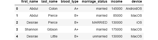
It is often the case that you will have some background information about your data. For example, let’s say you want to check for inconsistencies in the blood_type column of the above data frame. You find out beforehand that blood_type can only have these categories: [A+, A-, B+, B-, O+, O-, AB+, AB-]. So, you have to make sure that the column in the data source only includes these values.
In our case, there are 10k rows and visual search for inconsistencies is not an option, which is also the case for many other real-world data. Here is how can implement the best solution for such problems:
First, you should create a new data frame which holds all the possible values for a categorical column:

PRO TIP: It is a good practice to create such data frames which hold category mappings for each categorical column in the main data.
As we now have the correct categories in a separate data frame, we can use a basic set operation which gives us the difference of unique values in the two columns:
To get the difference between the two sets, we use .difference function. It basically returns all the values from the left set that are not in the right set. Here is a very simple example:
Attentive readers may have noticed that inside the set function, I also called .unique() on the blood_type. From what I have read from one StackOverflow thread, it seems that the time it takes to get the unique values will be much shorter if you use both set and unique for larger datasets.
Now, we will filter our main data for the blood types ‘C+’ and ‘D-’:
Using isin on blood_type will return a boolean series which we can use to index the data frame:
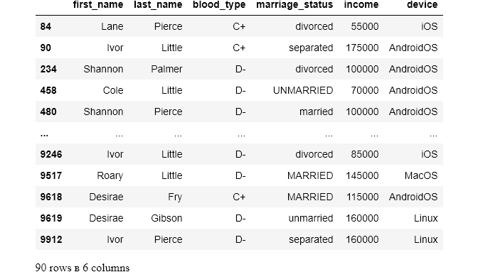
So, there are 90 individuals with incorrect blood types. Since we don’t have any clue of how these errors occurred (I did it😁😁😁), we have to drop them. It can be done in two ways:
As our column is clean now, it is safe to set it as a categorical variable:
Definitely check out the first part of this series. There, I covered basic and common data problems. You will also familiarize yourself with some of the functions I will be using here.
Value Inconsistency
Just like we talked about in the second section, there may be many representations of the same category in the data set. These errors may occur just because of simple typos, random capitalization, you name it. Continuing cleaning our data, the turn has come to the marriage_status column:
Using value_counts on a data frame column returns the count of unique values in that column. If you look at the result, you can immediately see the issues. The values should be either lower-case or upper-case. I prefer lower-case:
Using .str on a data frame column enables us to use all the Python string functions on each value of the column. Here, we are using .lower() which converts strings to lowercase.
value_counts is still returning 6 unique values, why? After paying close attention, you can see that one of the categories has extra leading whitespace. That's why it is being treated as an individual category. The same can be true for one of the unmarried, it might have trailing whitespace. We can use the string strip function to get rid of trailing whitespace from a string:
Now the column is clean. All is left is to convert this column into a category data type too:
Collapsing Data Into Categories
Sometimes, you may want to take already existing data, often numerical, and generate categories from it. This can be useful in a number of cases.
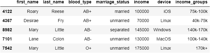
In our demographics dataset, we have an annual income column. It can be useful to cut this column into different income groups because doing so might give some extra insight into the data.
pandas has a perfect function for this: cut. It enables us to cut numerical ranges like data frame columns into bins and give them custom labels. Let's see it in action:
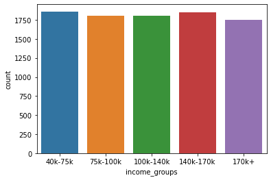
Now, we can use functions like value_counts to get more insight:
You can also plot a count plot:
Reducing the Number of Categories
Sometimes, there may be unnecessary categories. In such cases, you can collapse smaller categories into general and bigger categories which might suit your needs better. Consider the device column of our data:
It is not much use to compare phone’s operating system to computer’s. What would be better is to reduce the categories into mobileOS and desktopOS. To do this, first, we need to create a dictionary which maps each category to the new one:
Then, we use replace function of pandas which maps out the new categories dynamically:
If you liked the article, please share it and leave feedback. As a writer, your support means the world to me!
Read more articles related to the topic:


