Speeding up vision transformer prediction by 9 times with PyTorch, ONNX and TensorRT

How to use 16bit float, TensorRT, network rewriting and multi-threading to dramatically speed up deep learning model prediction

Vision transformer such as UNET, SwinUNETR are state-of-the-art in computer vision tasks, such as semantic segmentation. But it takes a lot of time for such models to make a prediction. This article shows how to speed up such model’s prediction by 9 times. This improvement paves the way for many real-time or near real-time applications.

The tumours segmentation task

To set the scene, I’m using the SwinUNETR model to segment lung tumours from chest CT scan images, which are single channel grayscale 3D images. Here is an example:

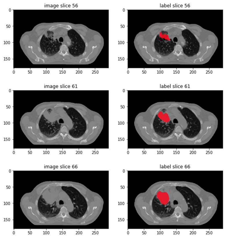
• Left column shows a few 2D slices from a 3D CT scan image, at the axial plane. The two crescent black areas are lungs.
• Right column shows the manual annotation of lung tumours.

Chest CT scans are typically sized 512×512×300, taking roughly 60 to 90 megabytes to store in disk. They are not small images.

I use PyTorch to train a SwinUNETR model to segment lung tumours. It takes around 10 seconds for a trained model to make a prediction on a chest CT scan. So 10 second per image is my starting point.

Before we go into speed optimization, let’s look at the model’s input and output, and how it makes predictions.

Model input and output shapes

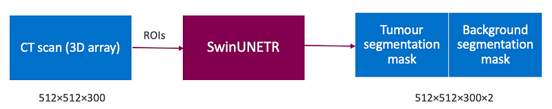
• The input is a 3D numpy array representing a chest CT scan.
• The SwinUNETR model couldn’t hold the whole image; it’s too big. A solution is to cut the image into smaller chunks, called Region of Interest (ROIs). In my setup, a region of interest is sized 96×96×96.
• The SwinUNETR model sees a single region of interest at a time, outputs two binary segmentation masks, one for the tumour class and the other for the background class. Both masks are of the region of interest size, so 96×96×96. More precisely, SwinUNETR outputs two unnormalized class probability masks. In a later step, these unnormalized masks are normalized into proper probabilities between 0 and 1 via softmax, and then argmax-ed into binary masks.
• These masks are merged according to how the corresponding regions of interest are cut to deliver two full size segmentation masks — the tumour mask and the background mask — each mask has the size of the whole chest CT scan. Note that even though the model returns two segmentation masks, we are only interested in the tumour mask, and will ignore the background mask.
• The input and output arrays, and the model, uses 32 bit floats.

Sliding window inference

The following pseudo code implements the above prediction idea.

Note code snippets in this article are pseudo code to keeps them succinct. Following the same argument, methods whose implementation is obvious, such as split_image, are left to your imagination.

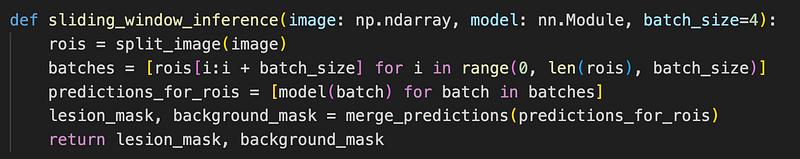
• The sliding_window_inference method accepts the full CT scan image and a PyTorch model. It also accepts a batch_size because a region of interest is small, and a GPU can hold multiple of them at a time for prediction. batch_size specifies how many regions of interest to send to the GPU. sliding_window_inference returns the binary tumour segmentation and background mask.
• The method first splits the whole image into regions of interest and then groups them into batches with each group containing batch_size regions of interest. Here I assume the number of regions of interest is dividable by batch_size for code simplicity.
• Each batch is sent to the model to make a batch of predictions. Each prediction is for a single region of interest.
• Finally predictions for all regions of interest are merged to form two full sized segmentation masks. The merging also includes softmax and argmax.

Snippet to make prediction for an image

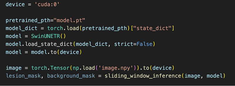
The following snippets calls the sliding_window_inference method to make a prediction for an image file loaded into the the first GPU “cuda:0” as a PyTorch tensor:

With the above setup, I now introduce a set of tactics to make the model predict faster.

Tactic 1: making prediction in 16bit floats

By default, the trained PyTorch model works with 32bit floating point. But often a 16bit float precision is enough to deliver very similar segmentation result. It is easy to turn a 32bit model into a 16bit one using just a single PyTorch API half:

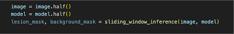
This tactic reduces the prediction time from 10 second to 7.7 second.

Tactic 2: converting model to TensorRT

TensorRT is a software from Nvidia that aims at delivering fast inference for deep learning models. It achieves this by converting a general model, such as a PyTorch model, or a TensorFlow model, which runs in many hardware into a TensorRT model that only runs in one particular hardware — the hardware that you ran the model conversion on. During the conversion, TensorRT also performs many speed optimizations.

The trtexec executable from the TensorRT installation performs the conversion. The problem is, sometimes, the conversion from a PyTorch model to a TensorRT model fails. It fails for me on the PyTorch SwinUNETR model. The particular failure message is not important, you will encounter your own errors.

The important thing is to know there is a walk-around. The walk-around is to first convert a PyTorch model into an intermediate format, ONNX, and then convert the ONNX model into a TensorRT model.

ONNX is an open format built to represent machine learning models. ONNX defines a common set of operators — the building blocks of machine learning and deep learning models — and a common file format to enable AI developers to use models with a variety of frameworks, tools, runtimes, and compilers.

The good news is that the support to convert an ONNX model into a TensorRT model is better than converting a PyTorch model into a TensorRT model.

Converting a PyTorch model to an ONNX model

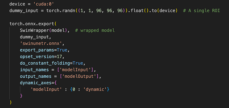
The following snippet converts a PyTorch model into an ONNX model:

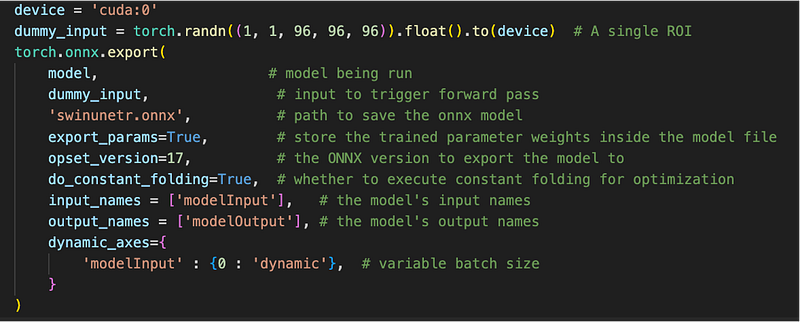
It first creates random input for a single region of interest. Then uses the export method from the installed onnx Python package to perform the conversion. This conversion outputs a file called swinunetr.onnx. The argument dynamic_axes specifies that the TensorRT model should support dynamic size at the 0th dimension of the input, that is, the batch dimension.

Converting a n ONNX model to a TensorRT model

Now we can invoke the trtexec command line tool to convert the ONNX model to a TensorRT model:

• the onnx=swinunetr.onnx command line option specifies the location of the onnx model.
• the saveEngine=swinunetr_1_8_16.plan option specifies the file name for the resulting TensorRT model, called a plan.
• the fp16 option requires that the converted model runs at 16 bit floating point precision.
• the minShapes=modelInput:1×1×96×96×96 specifies the minimal input size to the resulting TensorRT model.
• the maxshapes=modelInput:16×1×96×96×96 specifies the maximal input size to the resulting TensorRT model. Since during the PyTorch to ONNX conversion, we only allow the 0th dimension, that is, the batch dimension, to support dynamic size, here in minShapes and maxShapes, only the first number can change. Together they tells the trtexec tool to output a model that can be used for an input with the batch size between 1 and 16.
• the optShapes=modelInput:8×1×96×96×96 specifies that the resulting TensorRT model should run the fastest with a batch size of 8.
• the workspace=10240 option gives trtexec 10G of GPU memory to work on the model conversion.

trtexec will run for 10 to 20 minutes, and outputs the generated TensorRT plan file.

Making prediction using the TensorRT model

The following snippet loads the TensorRT model plan file and uses the TrtModel that is adapted from stackoverflow:

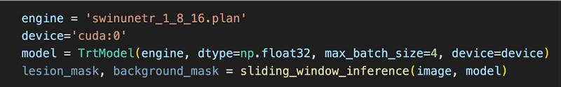
Note that even though in the trtexec command line, we specified the fp16 option, here when loading the plan, we still need to specify the 32 bit floating point. Strange.

Minor adaptations are needed in the TrtModel you got from stackoverflow, but you will work it out. It is not that difficult.

With this tactic, the prediction time is 2.89 second!

Tactic 3: Wrapping model to return one mask

Our SwinUNETR model returns two segmentation masks, one for tumour and one for background, in the form of unnormalized probabilities. These two masks are first transferred from GPU back to CPU. Then in CPU, these unnormalized probabilities are softmax-ed to proper probabilities between 0 and 1, and finally argmax-ed to generate binary masks.

Since we only use the tumour mask, there is no need for the model to return the background mask. Transferring data between GPU and CPU takes time, and computations such as softmax takes time.

To have a model that only returns a single mask, we can create a new class that wrappers the SwinUNETR model:

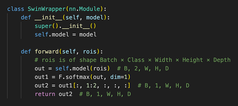
The following figure illustrates the new model input output:

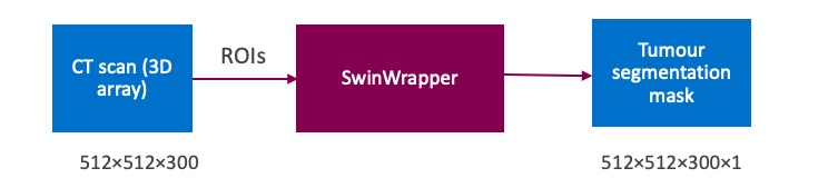
The forward method pushes a batch of input regions of interest through the forward pass of the neural network to make prediction. In this method:

• the original model is first called on the passed-in input regions of interest to get the predictions of the two segmentation classes. The output is of shape Batch×2×Width×Height×Depth because in the current tumour segmentation task, there are two classes — tumour and background. Result is stored in the out variable.
• Then softmax is applied to the two unnormalized segmentation masks to turn them into normalized probabilities between 0 and 1.
• Then only the tumour class, that is, class 1, is selected to return to the caller.

So, actually, this wrapper implements two optimizations:

1. only returns a single segmentation mask, instead of two.
2. moves the softmax operation from CPU into GPU.

What about the argmax operation? Since only one segmentation mask is returned, there is no need for argmax. Instead, to create the original binary segmentation mask, we will do tumour_segmentation_probability ≥ 0.5, with tumour_segmentation_probability being the result from the forward method in SwinWrapper.

Since SwinWrapper is a PyTorch model, we need to do the PyTorch to ONNX, and ONNX to TensorRT conversion steps again.

When converting the SwinWapper model to an ONNX model, it only change needed is to use wrapped model:

And the trtexec command line to convert an ONNX model to a TensorRT plan stay unchanged. So I won’t repeat it here.

This tactic reduced the prediction time from 2.89 second to 2.42 second.

Tactic 4: distributing regions of interest to multiple GPUs

All the above tactics uses only one GPU, but sometimes we want to use a more expensive multiple GPUs machine to deliver even faster predictions.

The idea is to load the same TensorRT model into n GPUs, and inside sliding_window_inference, we further split a batch of ROIs to n parts, and send each part to a different GPU. This way, the time-consuming forward pass of the SwinWrapper network can run concurrently for different parts.

We need to change the sliding_window_inference method into the following sliding_window_inference_multi_gpu:

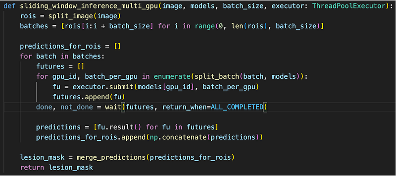
• Same as before, we group regions of interest in different batches.
• We split each batch into parts, depending on how many GPUs are given.
• For each part batch_per_gpu, we submit a task to into a ThreadPoolExecutor. The task performs model inference on the passed-in part.
• The submit method returns immediately with a future object, representing the result of the task when it finishes. It is crucial for the submit method to return immediately before the task finishes, so we can post other tasks to different threads without waiting, achieving parallelism.
• After all tasks submittedin the inner for loop, wait for all future objects to complete.
• After the tasks’ completion, read results from the futures and merge results.

To invoke this new version of sliding_window_inference_multi_gpu, use the following snippet:

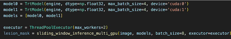
• Here I used two GPUs, so I created two TensorRT models, each into a different GPU, “cuda:0” and “cuda:1”.
• Then I created a ThreadPoolExecutor with two threads.
• I passed the models and the executor into the sliding_window_inference_multi_gpu method, similar to the case of a single GPU, to get the tumour class segmentation mask.

This tactic reduces the prediction time from 2.42 second to 1.38 second!

Now we have four tactics that improved the prediction speed of the SwinUNETR model by 9 times. That’s not too bad. But are we sacrificing prediction precision for speed?

Are we sacrificing prediction precision for speed?

Note here the word “precision” means how well the final model segment tumours, it does not mean the floating point prediction, for example, 16bit, 32bit precision.

To answer this question, we need to look at the DICE metric that measures the performance of a segmentation model.

A DICE score is calculated as the proportion of overlapping between the predicted tumour and the ground truth tumour. DICE score is between 0 and 1; a larger DICE score means a better model prediction:

• DICE 1 is perfect prediction,
• DICE 0 is completely wrong prediction, or no prediction at all.

Let’s look at the DICE score for a test image:

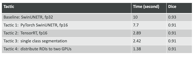
We can see that only when we turned a 32bit PyTorch model to a 16bit model in tactic 1, the DICE score slightly decreased from 0.93 to 0.91. Other tactics don’t decrease the DICE score. This shows that the tactics can achieve much faster prediction speed with only a tiny bit of precision loss.

Conclusions

This article introduces four tactics that can make vision transformer predict at a much faster speed by using tools such as ONNX, TensorRT and multi-threading.

Acknowledgement

I would like to give a big thank you to my friend Chunyu Jin. He introduced me to the possibilities of fast deep learning model inferences. He made the first running TensorRT SwinUNETR model for me and suggested many of the tactics that I tried out here.