
Making Sense of the Game of Thrones Universe Using Community Detection Algorithms
Community detection algorithms are accurate and surprisingly easy to use
More and more I’ve been working in graphs. Graphs are particularly useful when you are analyzing connection and community, and can be an extremely efficient way to store data. Sometimes I’ll use a graph database to get data just because it’s faster than a traditional relational database.
In this post I want to focus on community detection algorithms, which have a lot of practical uses. They can help identify a structure in a set of interactions, which has applications to organizational design, but can also be useful in other fields such as digital communications and crime investigation — for example, the famous Panama Papers investigation made major use of graphs and community detection.
What is community detection?
If communities exist inside a network, you’d expect that two nodes (eg people) who are more closely connected are more likely to be members of the same community. Working off this principle, a variety of algorithms exist that iterate through nodes and groups of nodes in networks and try to form an optimal grouping of the nodes, so that connections inside the groups are dense and connections between the groups are sparse.
Of course, large networks are complex, and so it’s usually quite impossible to find completely separate communities. Communities can overlap substantially, and algorithms are primarily concerned with optimizing. Visually, in these situations, it’s common for the end result to look a bit messy, but the visualization is not the point. Through performing community detection we get access to valuable information which can help us take action to improve efficiency. For example we may institute a formal organization structure which is more aligned with the true flow of work, or we might reconfigure server clusters to speed up information flow.
Game of Thrones network
To illustrate the power of community detection algorithms, I’m going to take the network of all character interactions in Game of Thrones, Seasons 1–8, and see what communities I can find. I’ve never watched the show, so have no idea how intuitive the results will be — maybe some readers can give a point of view after they’ve seen the results.
In this network, any two characters are connected if they have appeared in the same scene, and the strength of the connection is determined by the number of scenes they have appeared together in.
First — let’s build the network. Many thanks to Github user mathbeveridge who has created edgelists for the network for each season here: https://github.com/mathbeveridge/gameofthrones/tree/master/data. I’m going to just grab these edgelists straight from github and build them into one compiled edgelist to create the network using the igraph package in R.
library(tidyverse)
library(readr)
library(igraph)
# get s1 edgelist edgefile_url "https://raw.githubusercontent.com/mathbeveridge/gameofthrones/master/data/got-s1-edges.csv" edgelist <- readr::read_csv(edgefile_url) # append edglistists for s2-8
for (i in 2:8) {
edgefile_url <- paste0("https://raw.githubusercontent.com/mathbeveridge/gameofthrones/master/data//got-s", i, "-edges.csv") edges <- readr::read_csv(edgefile_url) edgelist <- edgelist %>%
dplyr::bind_rows(edges)
} seasons <- 1:8 # <- adjust if you want to focus on specific seasons edgelist <- edgelist %>%
dplyr::filter(Season %in% seasons) # create igraph network with weighted edges edgelist_matrix <- as.matrix(edgelist[ ,1:2]) got_graph <- igraph::graph_from_edgelist(edgelist_matrix, directed = FALSE) %>%
igraph::set.edge.attribute("weight", value = edgelist$Weight)OK, we’ve built our GoT network. Easy as that. Let’s take a quick look at it.
l <- igraph::layout_with_mds(got_graph)
plot(got_graph, vertex.label = NA, vertex.size = 5, rescale = F, layout = l*0.02)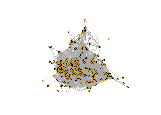
This looks like a pretty busy graph with lots of connections, and it’s hard to discern any meaningful or helpful structure to it. But it won’t take long for us to fix that.
Using the Louvain community detection algorithm
The Louvain community detection algorithm is a well-regarded algorithm for creating optimal community structures in complex networks. It is not the only one available (a fairly new algorithm called the Leiden algorithm is thought to perform slightly better), but there is an easy implementation of the Louvain algorithm in the igraph package, and so we can run the community detection with a fast, single line command. So let's do that and assign all our nodes to their respective community, and see what size our communities are
# run louvain with edge weights louvain_partition <- igraph::cluster_louvain(got_graph, weights = E(got_graph)$weight) got_graph$community <- louvain_partition$membership sizes(louvain_partition) %>% knitr::kable()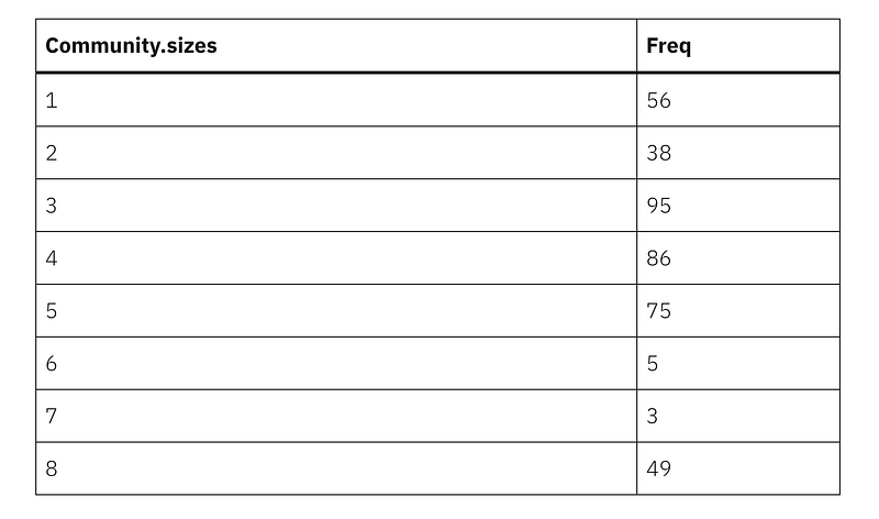
So we have a couple of very small communities here — lets take a look at who is in these.
membership(louvain_partition)[which(membership(louvain_partition) %in% c(6,7))]## BALON_DWARF ROBB_DWARF RENLY_DWARF STANNIS_DWARF JOFFREY_DWARF BLACK_JACK KEGS MULLY
## 6 6 6 6 6 7 7 7So a quick bit of online research suggests that these are one-off communities that appear in very specific episodes of GoT and who interact almost entirely with each other — the five dwarfs do a role play of the five kinfs in Season 4, and the trio on Black Jack, Kegs and Mully also appear in that same season. While it’s reassuring that these peripheral communities are being identified, its probably not helpful to consider them in the main questions we are looking at here, so I’ll keep them to one side as we proceed.
Characterizing the main communities
We will want to find a way to characterize our main communities. One way of doing that is to identify important nodes in each community — characters how are important in the overall connectedness of that community.
First we could find the nodes that have the most connection to other nodes inside each community. Let’s do that, by creating subgraphs of each community, and iterating a vector that contains the names of the nodes with the highest degree in each community.
high_degree_nodes <- c() for (i in 1:8) {
subgraph <- induced_subgraph(got_graph, v = which(got_graph$community == i)) degree <- igraph::degree(subgraph) high_degree_nodes[i] <- names(which(degree == max(degree))) }
high_degree_nodes[c(1:5, 8)]## [1] "DAENERYS" "SANSA" "CERSEI" "JON" "THEON" "ARYA"So we can see the six most connected characters are, unsurprisingly, leading characters, and they help us characterize the communities we have detected. We could also try to characterize each community by the node that is the best connector of other nodes — a measure called betweenness centrality.
high_btwn_nodes <- c() for (i in 1:8) { subgraph <- induced_subgraph(got_graph, v = which(got_graph$community == i)) btwn <- igraph::betweenness(subgraph) high_btwn_nodes[i] <- names(which(btwn == max(btwn))) }
high_btwn_nodes[c(1:5, 8)]## [1] "JORAH" "SANSA" "TYRION" "SAM" "ROBB" "ARYA"We can see that for a couple of communities the central character is the same with this measure, but for the rest it is different — which may help further characterize the community.
Visualizing the communities
It’s often helpful for people to look at a network, although for a network of this size that can be quite complex. By color coding the nodes and edges in the communities, we can better differentiate them, and we can then also label the nodes of the most central characters. Another option is to scale the nodes size to the importance of the node in the overall network.
First we can generate a pretty sphere network.
# give our nodes some properties, incl scaling them by degree and coloring them by community V(got_graph)$size <- degree(got_graph)/10
V(got_graph)$frame.color <- "white"
V(got_graph)$color <- got_graph$community
V(got_graph)$label <- V(got_graph)$name # also color edges according to their starting node edge.start <- ends(got_graph, es = E(got_graph), names = F)[,1] E(got_graph)$color <- V(got_graph)$color[edge.start] E(got_graph)$arrow.mode <- 0 # only label central characters v_labels <- which(V(got_graph)$name %in% high_degree_nodes[c(1:5, 8)]) for (i in 1:length(V(got_graph))) {
if (!(i %in% v_labels)) {
V(got_graph)$label[i] <- ""
}
} # plot network l1 <- layout_on_sphere(got_graph)
plot(got_graph, rescale = F, layout = l1)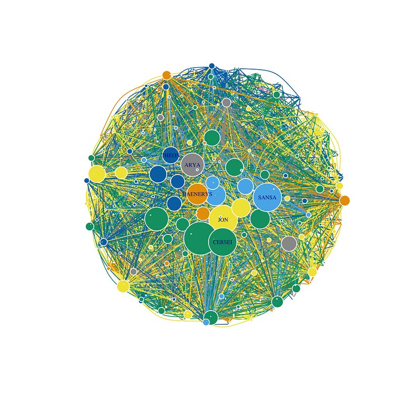
This is pretty, but not helpful in visualizing the separate communities. For this it’s better to use a multi-dimensional scaling, to ensure that more distant nodes are less connected.
l2 <- layout_with_mds(got_graph)
plot(got_graph, rescale = F, layout = l2*0.02)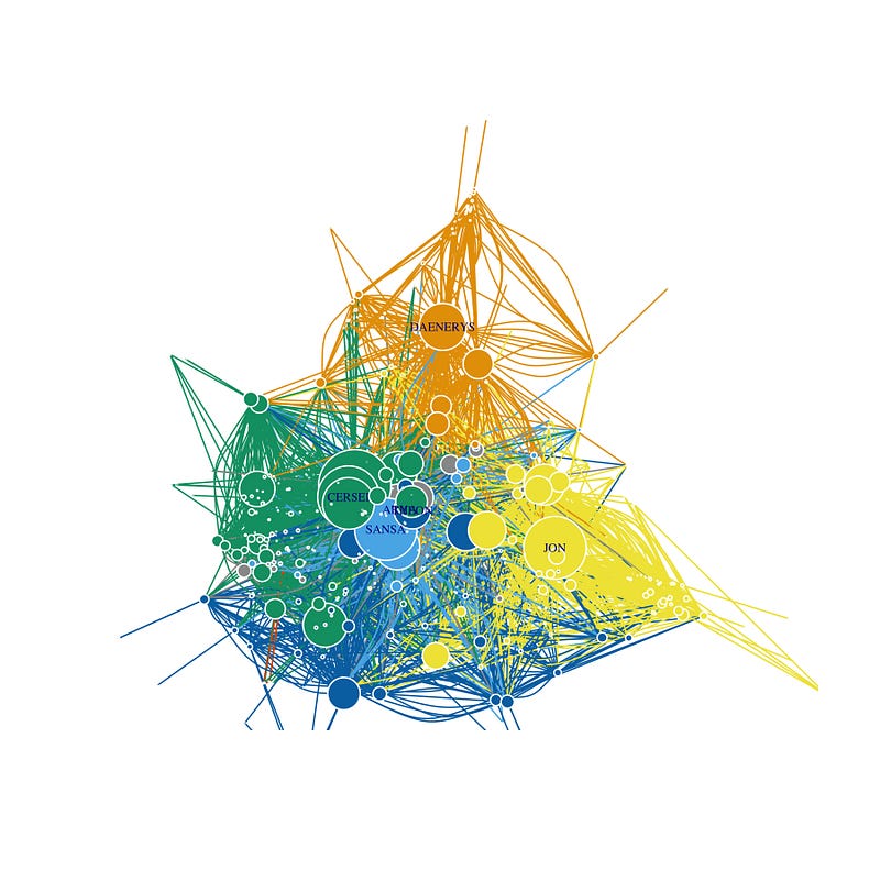
Nice! Of course there is a lot more we can do here to analyze and characterize the communities, but I wanted you to see that its pretty easy to implement this type of analysis in a few lines of code, and the ability of these algorithms to detech genuine communities is quite something! I’d encourage you to think about uses for this type of technology in your work or study. Do drop a comment if you can think of good uses for this.
Originally I was a Pure Mathematician, then I became a Psychometrician and a Data Scientist. I am passionate about applying the rigor of all those disciplines to complex people questions. I’m also a coding geek and a massive fan of Japanese RPGs. Find me on LinkedIn or on Twitter. Also check out my blog on drkeithmcnulty.com.


