Machine Learning Theory and Programming — Supervised Learning: Neural Networks

An introduction to popular machine learning algorithms

Machine learning is a method of data analysis that automates analytical model building. While artificial intelligence is the broad science of how to mimic human cognitive functions, machine learning is a specific subset that trains a machine to learn. Neural networks reflect the behavior of the human brain, allowing computer programs to recognize patterns and solve common problems.

In a previous article, we have defined supervised learning and unsupervised learning. The training data for supervised learning have correct answers, while unsupervised learning do not. Neural networks can solve both supervised and unsupervised problems. In this article, we are going to focus on supervised neural networks.

Neural Network Theory

A neural network is a network or circuit of neurons that is composed of artificial neurons, which are also called nodes. The terminology and structure are simulated by the human brain where biological neurons signal to each other.

Artificial neurons were first proposed in 1943 by Warren McCulloch and Walter Pitts in A logical calculus of the ideas immanent in nervous activity.

The concept of a neural network was first proposed in 1948 by Alan Turing in Intelligent Machinery.

Neural networks are computational models, which are capable of extracting meaning from imprecise or complex data. The learning process finds patterns and detects trends, similar to how the human brain works.

A neural network contains an input layer, zero or more hidden layers, and an output layer. Each layer has one or more nodes. Each node connects to the nodes in the next layer, and each connection has an associated weight. Starting from input nodes, a neural network produce an output, which is the solution of a problem.

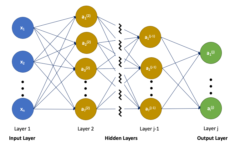
In the above graph, there are inputs x₁, x₂, …, xₙ. It goes through hidden layers from layer 2 to layer j -1, and produces outputs a₁⁽ʲ⁾, a₂⁽ʲ⁾, …, aᵢ⁽ʲ⁾, where aᵢ⁽ʲ⁾ is node i in layer j. Each layer can have different number of nodes.

Commonly, a bias node (a constant, typically initialized to 1) is added to each input layer to shift the activation function, which defines the output of a node given an input or a set of inputs.

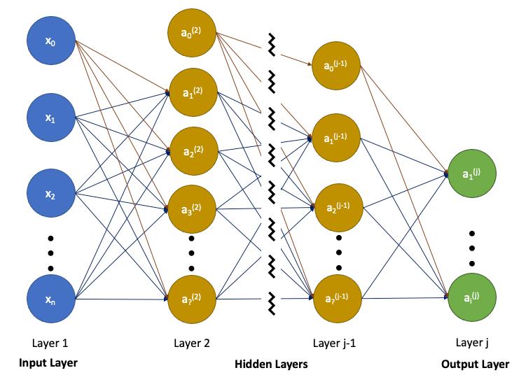
In the above graph, bias nodes are x₀, a₀⁽²⁾, …, a₀⁽ʲ⁻¹⁾. In fact, the input vector, x, is a special case of a⁽¹⁾.

We define the connection weight as Θᵢⱼ, each layer’s output is calculated forwardly by an activation function, f. The output of node i in layer j can be calculated as follows, if the previous layer has k nodes:

aᵢ⁽ʲ⁾ = f(Θᵢ₀⁽ʲ⁻¹⁾a₀⁽ʲ⁻¹⁾ + Θᵢ₁⁽ʲ⁻¹⁾a₁⁽ʲ⁻¹⁾ + ... + Θᵢₖ⁽ʲ⁻¹⁾aₖ⁽ʲ⁻¹⁾)

The activation function can be linear or nonlinear. When it is linear, the output is simply defined as follows:

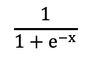
aᵢ⁽ʲ⁾ = Θᵢ₀⁽ʲ⁻¹⁾a₀⁽ʲ⁻¹⁾ + Θᵢ₁⁽ʲ⁻¹⁾a₁⁽ʲ⁻¹⁾ + ... + Θᵢₖ⁽ʲ⁻¹⁾aₖ⁽ʲ⁻¹⁾

When it is nonlinear, f could be a logistic function for a classification problem:

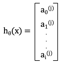
Hypothesis (h) is a mathematical model that best maps inputs (x) to outputs (y).

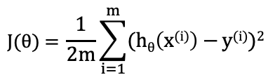
Cost function (J) is a mechanism that returns the error between the predicted outcomes (h) and the actual outcomes (y).

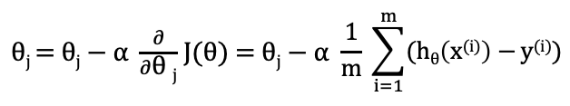
Gradient descent is an optimization algorithm that is used to compute coefficients to minimize the cost function. For every j = 0, 1, …, m, θⱼ is calculated iteratively using the following equation, where α is the learning rate.

These formulas are true for linear regression, polynomial regression, and logistic regression. It also applies to neural networks.

We train a neural network by fitting the weight, θ. For a given supervised dataset, (x, y), it is typically split into different sets:

Training set: It is part of dataset that is used for learning to calculate the weight. Typically, 60% of a dataset is used for training.
Validation set: It is part of dataset that is used to tune the parameters, such as, the number of hidden layers, the number of nodes on each layer, activation function, etc. Typically, 20% of a dataset is used for validation.
Test set: It is part of dataset that is used to assess the performance of a fully-trained model. Typically, 20% of a dataset is used for testing.

Neural Network Programming

For neural networks, computation algorithms are mathematically complicated. It is not very easy if we construct the model by ourselves.

There are machine learning specific programming languages, such as MATLAB, Octave, R, etc. For some of the general-purposed programming languages, such as Python, they are supplied with machine learning libraries. Therefore, it may only take one function call to train a model.

MATLAB is a proprietary multi-paradigm programming language and numeric computing environment developed by MathWorks. It provides a number of builtin functions for neural networks. feedforwardnet returns a feedforward neural network with specified hidden layer size and training function.

A feedforward network consists of a series of layers. The first layer has a connection from the network input. Each subsequent layer has a connection from the previous layer. The final layer produces the network’s output.

feedforwardnet supports a number of training functions. The default function is 'trainlm', which is Levenberg-Marquardt algorithm for nonlinear least-squares.

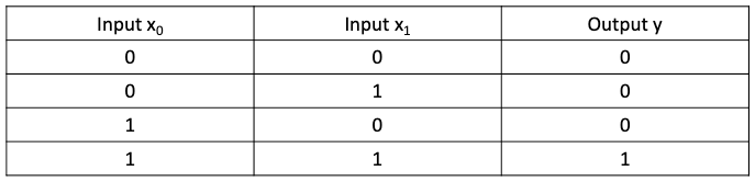
We train a neural network to perform the logical and operation, which produces the output, y, based on the input, x₀ and x₁.

Training & Testing Program

Here is the MATLAB program, where a training set is used to fit a neural network, and a test set is used to verify the neural network.

Line 1 specifies the function name, neuralNetwork, and the return value, output.

Lines 3–8 creates a training set using random numbers.

Line 3 sets the training set size to be 10.

Line 4 generates the input value, x. Here is one example:

Lines 5–8 generate the output value, y, based on the inputs, x₀ and x₁.

Line 11 creates a neural network, net, with 2 hidden layers.

Line 12 uses training set to fit the neural network, net.

Line 15 creates a test set of size 4, [0.01, 0.02; 0.4, 0.6; 0.8, 0.1; 0.9, 0.9]

Line 16 produces the prediction of the test set.

Here is the trained neural network, net:

Line 18 terminates the function.

Bias, Variance, and Training Set Size

The goal of supervised machine learning is to best estimate the mapping for the output value, y, based on the input, x. Cost function (J) measures the error between the predicted outcomes (h) and the actual outcomes (y). There are three types of errors:

Bias: It is an error from erroneous assumptions in the learning algorithm. High bias can cause an algorithm to miss the relevant relations between features and target outputs (underfitting).
Variance: It is an error from sensitivity to small fluctuations in the training set. High variance may result from an algorithm modeling the random noise in the training data (overfitting).
Irreducible: It is the error from misrepresentation of the problem. It cannot be reduced regardless of what algorithm is chosen.

If a learning algorithm is suffering from high bias, increasing the training set size will not help much. If learning algorithm is suffering from high variance, increasing the training set size will likely to help.

We use the test set, [0.01, 0.02; 0.4, 0.6; 0.8, 0.1; 0.9, 0.9]. The ideal result is [0 0 0 1].

We have used training set size of 10. The result is [-0.9973 0.1142 -0.9656 1.0639]. The error is obvious. The result of each run varies.

Increase the training set size to 100, and result is [-0.1039 0.2991 -0.0009 0.8526].

Increase the training set size to 1,000, and result is [-0.0162 0.0997 -0.1453 1.0463].

Increase the training set size to 10,000, and result is [-0.0175 0.4074 -0.0041 1.0546].

Obviously, after the 1000 training set’s fitting, increasing the training set size will not help much any more. Our example does not have noise, the modal is underfitting if the training set size is too small.

There is also another dimension to tune neural network. A smaller neural network with less nodes and hidden layers is computationally cheaper, and is more prone to underfitting. A larger neural network with more nodes and hidden layers is computationally more expensive, and is more prone to overfitting.

Conclusion

There are many machine learning algorithms. We have presented supervised neural networks in this article. Machine learning programming languages are designed with pre-built libraries and advanced support of data science and data models. We have showed an examples to train a neural network to perform a logical and operation. MATLAB’s builtin function, feedforwardnet, makes the training easy and effective.

Here is a list of other machine learning algorithms:

Thanks for reading. I hope this was helpful. If you are interested, check out my other Medium articles.

Note: Thanks, Josh Poduska, Andrew Ziegler, and Subir Mansukhani, for recommending machine learning resources! Also, thanks to Professor Andrew Ng’s Machine Learning Class.