Machine Learning Must Know — From Raw to Training Data

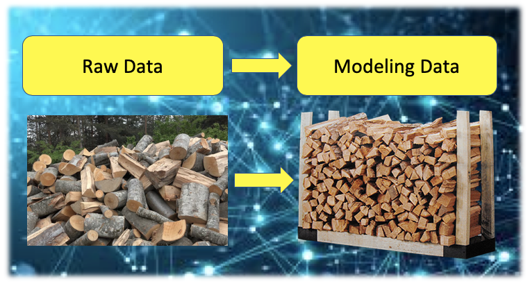
This topic seems too rudimentary, yet I found most machine learning books do not cover. Most machine learning books cover the techniques to split the modeling data randomly into training, test and validation datasets, then the topics quickly turn into k-fold cross-validation. But wait, how do we prepare the modeling data? The number of transactions of a credit card company can be billions, but that’s raw data not modeling data. The number of mortgage loan applicants can be millions. But you cannot use the raw data to build a model. So how do you prepare the modeling data from the raw data? Often the success of a data science project is determined by how the training data are defined. So I decided to write an article to talk about it in depth. I will use the mortgage default case as an example in this article.

This article is related to “Feature Engineering for Credit Card Fraud Detection” or “Feature Engineering for Healthcare Fraud Detection”. Fraud detection is a critical function to detect fraud early and prevent loss. You do not use the billions of raw transactions, as they are, to build a model. The raw data need to be prepared into modeling data to build a fraud detection model.

I have written articles on a series of data science topics. For ease of use, you can bookmark my summary post “Dataman Learning Paths — Build Your Skills, Drive Your Career” that lists the links to all articles.

What Are Raw Data?

Raw data are the original data. Figure (A) shows an example of customer records. There are three columns but you do not use the columns as variables for modeling purposes. Intelligence has to be derived from the raw data. That step is called feature engineering. The feature engineering varies by industry and relies on the business domain knowledge. See “Feature Engineering for Credit Card Fraud Detection” or “Feature Engineering for Healthcare Fraud Detection”.

Model Prediction Gives You an Educated Guess

You probably have heard “the past predicts the future”. We prepare the modeling data from past records to find the patterns in the data. These patterns are applied to the current data to predict the future. Modeling gives you an educated guess. Any event that has not happened in the past is hard to pattern in the model to predict the future (although the model can exploit any hidden or interaction patterns, but still not likely). So in this sense, a model provides a limited educated guess.

What Is the Objective of the Prediction?

You may want to know: “ Will a homeowner renew his home insurance policy next year (Yes or No)?” Or “How much should we charge a customer’s homeowner policy?” Or “How long will a customer continue to hold the homeowner's policy? These questions concern “if”, “how much” and “how long”.

The business objective will determine your selection for the target variable. If it is about “if yes or not”, your target variable is a binary “yes” or “no”. If the business objective is about “how much”, your target variable is the monetary amount. If it is about “how long”, your target variable is “the number of months”. You will also adopt the right algorithm, such as logistic regression, decision trees, or survival analysis to model.

The same thinking process can be applied to loan applications: “Will a mortgage loan applicant default in the future?” or to e-commerce: “Will a customer purchase again?” and many other cases.

How to Build the Modeling Dataset?

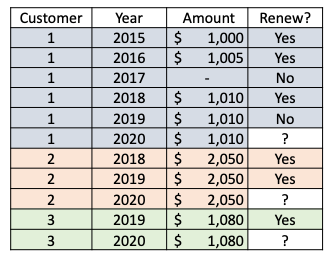
The business objectives will also shape your modeling dataset. All the above questions focus on the individual customer level, so the data should be better organized to the individual customer level to answer that question. In Figure (A), a customer has multiple records. Figure (B) collapses Figure (A). It is one customer per record. This is the grain or the minimum level of the data. It defines the right granularity of the data to build your machine-learning model.

Let’s give a summary of the grain of the data. If your business objective is to provide a prediction for each customer, the grain of the data is the customer level. Each record is a customer, as shown in Figure (B). If hypothetically your business objective is to provide predictions for a customer for each of multiple years, the grain of the data shall be at the customer and year level like Figure (A).

Again, Let’s Define the Modeling Dataset

Assume now is the end of 2019 as indicated by the green arrow in Figure (B). You need to develop a model to predict which customer will renew his homeowner policy in 2020. The green ellipses show your objective: you want to build a model to predict the responses in 2020, i.e., you want to use the blue Xs to predict the blue Y in 2020.

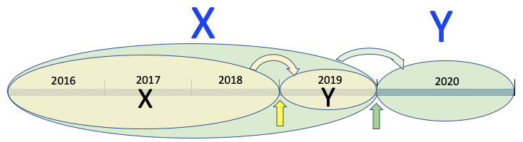
How do you define the modeling dataset? You can roll back one year as if you are at the end of 2018 (the yellow arrow). You can take the data in the previous years (the yellow ellipse) to build the model. You use data in 2016–2018 to create your black predictors Xs, and the responses in 2019 as your black target Y. In the modeling dataset, all the Xs are information up to the end of 2018.

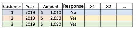
This is the modeling dataset that you split randomly into training, test and validation datasets, or k-fold cross-validation. This is what I talked about at the beginning of the article: most textbooks jump into training-test-validation for model training. Here I supplement the step from raw data to modeling data.

How to Prepare New Data for Prediction?

How do you apply this model to predict 2020? You will need to prepare the blue predictors Xs. The way you prepare your black Xs will be the way you prepare your blue predictors.

“Using the previous years to build the model relies on the assumption that there is no change year over year,” you may argue! Yes, you are right. Therefore this is an important point in selecting the right modeling data. If there is a dramatic change year over year, you are advised not to take old data to build your model.

An Example

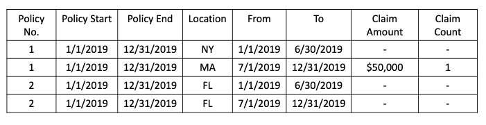
The following example is from my article “A Primer to Auto Insurance Pricing for Data Scientists”. To build a model to determine the insurance rates, various data sources including policy data, claims data, and external data are joined. Figure (D) shows the idea sources.

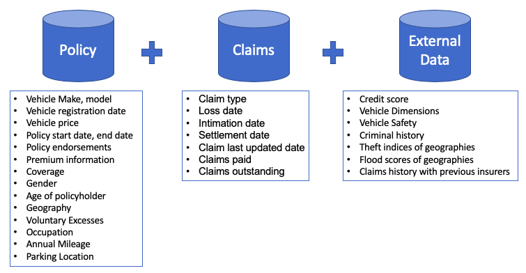
All the various data sources are joined to the policy-year level. The policy-year level can be at other desired levels such as monthly, quarterly, or half-yearly. Sometimes it makes a better sense to prepare the data at the policy-half-year level. Figure (E) presents this case. Notice that Policyholder 1 lived in New York in the first half of the policy year and then moved to Massachusetts in the second half of the policy year. The modeling dataset is set at a policy-half-year level in order to reflect the fact that policyholders moving from one location to another during a policy year.