Building a Machine Learning Recommendation Model from Scratch
Build a machine learning model for recommending the crew size for cruise ship buyers in Python

In this tutorial, we build a regression model using the cruise_ship_info.csv dataset for recommending the crew size for potential cruise ship buyers. This tutorial will highlight important data science and machine learning concepts such as:
a) data preprocessing and variable selection
b) basic regression model building
c) hyperparameters tuning
b) model evaluation
d) techniques for dimensionality reduction
The code for building this recommender system can be found on GitHub.
1. Import necessary libraries
import numpy as np
import pandas as pd
import matplotlib.pyplot as plt
import seaborn as sns
2. Read dataset and display columns
df=pd.read_csv("cruise_ship_info.csv")
df.head()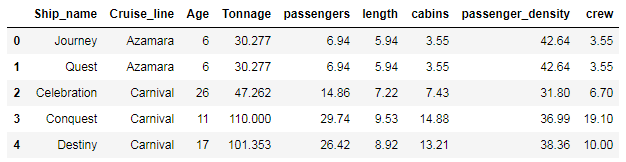
3. Calculate basic summary statistics for the dataset
df.describe()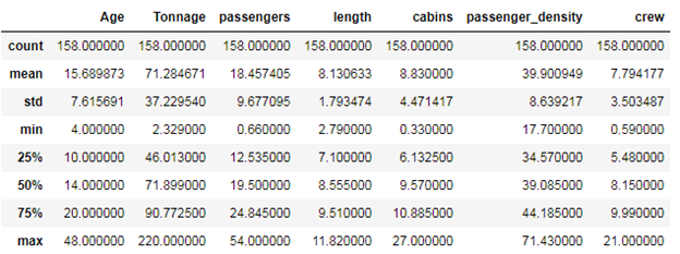
4. Generate scatter pair plot
cols = ['Age', 'Tonnage', 'passengers', 'length', 'cabins','passenger_density','crew']
sns.pairplot(df[cols], size=2.0)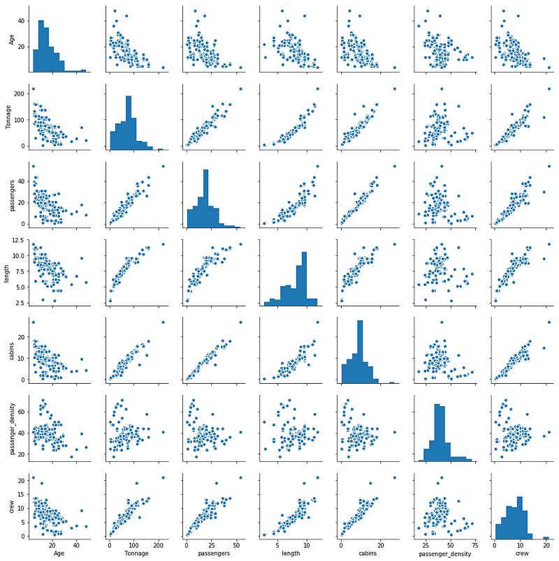
Observations from part 4:
1) We observe that variables are on different scales, for sample the Age variable ranges from about 16 years to 48 years, while the Tonnage variable ranges from 2 to 220. It is therefore important that when a regression model is built using these variables, variables be brought to the same scale either by standardizing or normalizing the data.
2) We also observe that the target variable ‘crew’ correlates well with 4 predictor variables, namely, ‘Tonnage’, ‘passengers’, ‘length’, and ‘cabins’.
5. Variable selection for predicting “crew” size
5a. Calculation of covariance matrix
cols = ['Age', 'Tonnage', 'passengers', 'length', 'cabins','passenger_density','crew']
from sklearn.preprocessing import StandardScaler
stdsc = StandardScaler()
X_std = stdsc.fit_transform(df[cols].iloc[:,range(0,7)].values)
cov_mat =np.cov(X_std.T)
plt.figure(figsize=(10,10))
sns.set(font_scale=1.5)
hm = sns.heatmap(cov_mat,
cbar=True,
annot=True,
square=True,
fmt='.2f',
annot_kws={'size': 12},
yticklabels=cols,
xticklabels=cols)
plt.title('Covariance matrix showing correlation coefficients')
plt.tight_layout()
plt.show()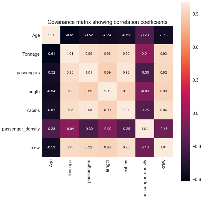
5b. Selecting predictor and target variables
From the covariance matrix plot above, we see that the “crew” variable correlates strongly with 4 predictor variables: “Tonnage”, “passengers”, “length, and “cabins”.
cols_selected = ['Tonnage', 'passengers', 'length', 'cabins','crew']df[cols_selected].head()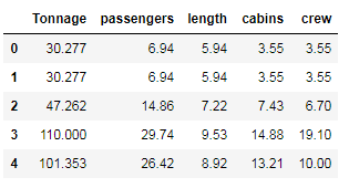
X = df[cols_selected].iloc[:,0:4].values    # features matrix
y = df[cols_selected]['crew'].values        # target variable
6. Data partitioning into training and testing sets
from sklearn.model_selection import train_test_split
X = df[cols_selected].iloc[:,0:4].values
y = df[cols_selected]['crew']
X_train, X_test, y_train, y_test = train_test_split( X, y, test_size=0.4, random_state=0)
7. Building a multi-regression model
Our machine learning regression model for predicting a ship’s “crew” size can be expressed as:
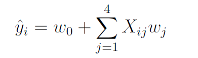
from sklearn.linear_model import LinearRegression
slr = LinearRegression()slr.fit(X_train, y_train)
y_train_pred = slr.predict(X_train)
y_test_pred = slr.predict(X_test)plt.scatter(y_train_pred, y_train_pred - y_train,
c='steelblue', marker='o', edgecolor='white',
label='Training data')
plt.scatter(y_test_pred, y_test_pred - y_test,
c='limegreen', marker='s', edgecolor='white',
label='Test data')
plt.xlabel('Predicted values')
plt.ylabel('Residuals')
plt.legend(loc='upper left')
plt.hlines(y=0, xmin=-10, xmax=50, color='black', lw=2)
plt.xlim([-10, 50])
plt.tight_layout()
plt.legend(loc='lower right')
plt.show()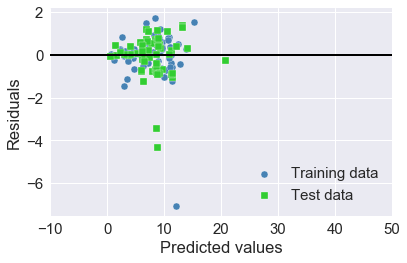
7a. Evaluation of regression model
from sklearn.metrics import r2_score
from sklearn.metrics import mean_squared_error
print('MSE train: %.3f, test: %.3f' % (
mean_squared_error(y_train, y_train_pred),
mean_squared_error(y_test, y_test_pred)))
print('R^2 train: %.3f, test: %.3f' % (
r2_score(y_train, y_train_pred),
r2_score(y_test, y_test_pred)))MSE train: 0.955, test: 0.889
R^2 train: 0.920, test: 0.9287b. Regression coefficients
slr.fit(X_train, y_train).intercept_-0.7525074496158393slr.fit(X_train, y_train).coef_array([ 0.01902703, -0.15001099, 0.37876395, 0.77613801])8. Feature Standardization, Cross-Validation, and Hyperparameter Tuning
from sklearn.metrics import r2_score
from sklearn.model_selection import train_test_split
X = df[cols_selected].iloc[:,0:4].values
y = df[cols_selected]['crew']
from sklearn.preprocessing import StandardScaler
sc_y = StandardScaler()
sc_x = StandardScaler()
y_std = sc_y.fit_transform(y_train[:, np.newaxis]).flatten()
train_score = []
test_score = []for i in range(10):
X_train, X_test, y_train, y_test = train_test_split( X, y, test_size=0.4, random_state=i)
y_train_std = sc_y.fit_transform(y_train[:, np.newaxis]).flatten()
from sklearn.preprocessing import StandardScaler
from sklearn.decomposition import PCA
from sklearn.linear_model import LinearRegression
from sklearn.pipeline import Pipeline
pipe_lr = Pipeline([('scl', StandardScaler()),('pca', PCA(n_components=4)),('slr', LinearRegression())])
pipe_lr.fit(X_train, y_train_std)
y_train_pred_std=pipe_lr.predict(X_train)
y_test_pred_std=pipe_lr.predict(X_test)
y_train_pred=sc_y.inverse_transform(y_train_pred_std)
y_test_pred=sc_y.inverse_transform(y_test_pred_std)
train_score = np.append(train_score, r2_score(y_train, y_train_pred))
test_score = np.append(test_score, r2_score(y_test, y_test_pred))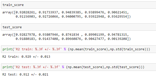
9. Techniques of Dimensionality Reduction
9a. Principal Component Analysis (PCA)
train_score = []
test_score = []
cum_variance = []for i in range(1,5):
X_train, X_test, y_train, y_test = train_test_split( X, y, test_size=0.4, random_state=0)
y_train_std = sc_y.fit_transform(y_train[:, np.newaxis]).flatten()
from sklearn.preprocessing import StandardScaler
from sklearn.decomposition import PCA
from sklearn.linear_model import LinearRegression
from sklearn.pipeline import Pipeline
pipe_lr = Pipeline([('scl', StandardScaler()),('pca', PCA(n_components=i)),('slr', LinearRegression())])
pipe_lr.fit(X_train, y_train_std)
y_train_pred_std=pipe_lr.predict(X_train)
y_test_pred_std=pipe_lr.predict(X_test)
y_train_pred=sc_y.inverse_transform(y_train_pred_std)
y_test_pred=sc_y.inverse_transform(y_test_pred_std)
train_score = np.append(train_score, r2_score(y_train, y_train_pred))
test_score = np.append(test_score, r2_score(y_test, y_test_pred))
cum_variance = np.append(cum_variance, np.sum(pipe_lr.fit(X_train, y_train).named_steps['pca'].explained_variance_ratio_))plt.scatter(cum_variance,train_score, label = 'train_score')
plt.plot(cum_variance, train_score)
plt.scatter(cum_variance,test_score, label = 'test_score')
plt.plot(cum_variance, test_score)
plt.xlabel('cumulative variance')
plt.ylabel('R2_score')
plt.legend()
plt.show()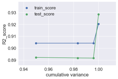
Observations from part 9a:
We observe that by increasing the number of principal components from 1 to 4, the train and test scores improve. This is because, with fewer components, there is a high bias error in the model, since the model is overly simplified. As we increase the number of principal components, the bias error will reduce, but complexity in the model increases.
9b. Regularized Regression: Lasso
from sklearn.model_selection import train_test_split
X_train, X_test, y_train, y_test = train_test_split( X, y, test_size=0.4, random_state=0)
y_train_std = sc_y.fit_transform(y_train[:, np.newaxis]).flatten()
X_train_std = sc_x.fit_transform(X_train)
X_test_std = sc_x.transform(X_test)
alpha = np.linspace(0.01,0.4,10) #lasso parametersfrom sklearn.linear_model import Lasso
lasso = Lasso(alpha=0.7)r2_train=[]
r2_test=[]
norm = []
for i in range(10):
lasso = Lasso(alpha=alpha[i])
lasso.fit(X_train_std,y_train_std)
y_train_std=lasso.predict(X_train_std)
y_test_std=lasso.predict(X_test_std)
r2_train=np.append(r2_train,r2_score(y_train,sc_y.inverse_transform(y_train_std)))
r2_test=np.append(r2_test,r2_score(y_test,sc_y.inverse_transform(y_test_std)))
norm= np.append(norm,np.linalg.norm(lasso.coef_))plt.scatter(alpha,r2_train,label='r2_train')
plt.plot(alpha,r2_train)
plt.scatter(alpha,r2_test,label='r2_test')
plt.plot(alpha,r2_test)
plt.scatter(alpha,norm,label = 'norm')
plt.plot(alpha,norm)
plt.ylim(-0.1,1)
plt.xlim(0,.43)
plt.xlabel('alpha')
plt.ylabel('R2_score')
plt.legend()
plt.show()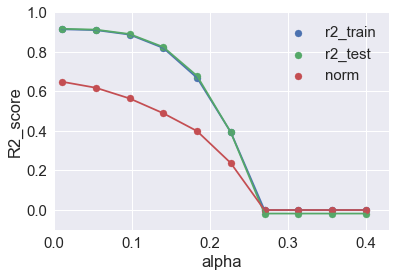
Observations from part 9b:
We observe that as the regularization parameter alpha increases, the norm of the regression coefficients become smaller and smaller. This means more regression coefficients are forced to zero, which intend to increases bias error (oversimplification). The best value to balance bias-variance tradeoff is when alpha is kept low, say alpha = 0.1 or less.
Summary
In summary, we’ve shown how a simple regression model can be built using the cruise_ship_info.csv dataset for predicting the crew size for potential ship buyers. The code for this recommendation system can be found on GitHub.
References
- Raschka, Sebastian, and Vahid Mirjalili. Python Machine Learning, 2nd Ed. Packt Publishing, 2017.
- Benjamin O. Tayo, Machine Learning Model for Predicting a Ships Crew Size, https://github.com/bot13956/ML_Model_for_Predicting_Ships_Crew_Size.