How Does Gradient Descent Works? | Towards AI

Machine Learning: How the Gradient Descent Algorithm Works

Most machine learning algorithms perform predictive modeling by minimizing an objective function, thereby learning the weights that must be applied to the testing data in order to obtain the predicted labels. The simplest objective (loss) function is the Sum of Squared Errors (SSE) function which we will denote as J(w):

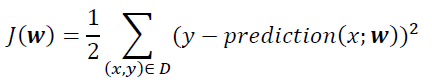
Here, x represents the features, y the labels, D the training dataset containing features and labels, and w are the weights learned from the model by minimizing the objective function. The objective function is often minimized using the gradient descent (GD) algorithm. In the GD method, the weights are updated according to the following procedure:

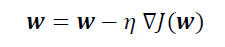
i.e., in the direction opposite to the gradient. Here, eta is a small positive constant referred to as the learning rate.

But why does the GD algorithm work?

Why the GD algorithm works

To illustrate, we consider a simple example, namely, the 2D Gaussian function. We perform calculations using Mathematica software.

Plot3D[Exp[-(x² + y²)], {x, -2, 2}, {y, -2, 2}, PlotRange -> All]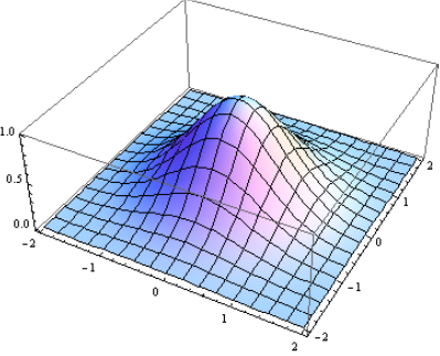

We see that the function has a maximum value at (0,0). Now let us generate a contour plot of the function and superimpose on it the unit vector in the direction of the gradient vector:

p1 = ContourPlot[Exp[-(x² + y²)], {x, -2, 2}, {y, -2, 2}];

p2 = VectorPlot[{-x/Sqrt[x² + y²] , -y/Sqrt[x² + y²]}, {x, -2,2}, {y, -2, 2}];

Show[p1, p2]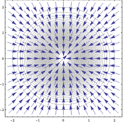

We observe that the vector fields of the unit vectors (arrows) of the gradient point towards the origin (0,0), where the function attains its maximum value. So we see that the gradient vector always points in the direction of the maximum of a function.

Hence the following rules apply:

1. To Maximize a function of several variables, we take steps in the direction of the gradient vector.
2. To Minimize a function of several variables, we take steps opposite the direction of the gradient vector.

Example of GD algorithm

Suppose we want to minimize the objective function:

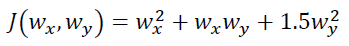
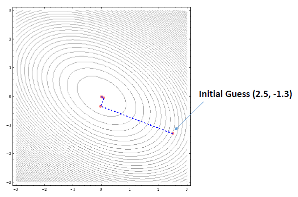
Clearly, this function has a global minimum of 0 at the point (w_x =0, w_y = 0). Applying the GD algorithm with some initial guess (w_x = 2.5, w_y = -1.3), we can show with a few lines of code that the algorithm converges to the correct minimum, that is to the point (0,0), as shown here:

In summary, we have shown how the GD algorithm works using a very simple example. If you would like to see how the GD algorithm is used in a real machine learning classification algorithm, see the following repository: https://github.com/bot13956/LogisticRegression_gradient_descent

For more information about the GD algorithm, see the following book: “Python Machine Learning” by Sebastian Raschka (Chapter 2 & 3).

Thanks for reading.