
Machine learning beats BTC/USDT on unseen data, even with transaction fees and slippage.
How physics research turned into AI modelling, turned into crypto trading.

Preface
There are a lot of articles about experimentation applying machine learning to crypto trading but it is hard to find one with realistic methodology. Ideally, results should come either from trading history on an actual exchange or from a simulation with unseen data and included transaction fees. That’s why I wrote this article — I want to tell you how I do my financial market research, present some of its findings and eventually show you actual results. All with assumptions grounded in reality — including transaction fees, slippage and unseen data.
Seeing what doesn’t work
I used to work on various physics experiments — most notably in the ATLAS project at CERN (using Large Hadron Collider, world’s largest and highest-energy particle collider and the largest machine in the world). I came there as a physics student and became a data scientist taking on event topology classification problems. In summer 2018 my interest in trading stocks started. I knew my data science intuition and programming skills could be useful, so the idea to use mathematical models with some automation came up very naturally. I spent the summer looking for useful articles but it was very difficult to find something interesting. If someone claimed something works I couldn’t reproduce it in any way.
I read around a hundred articles regarding machine learning in finance in the last 1.5 years. I’ve seen people using LSTMs, path integrals, all kinds of reinforcement learning but I didn’t find anything exceptional performance-wise. Still, it is useful to see what doesn’t work so you don’t have to waste time trying it yourself.
Market behaviour
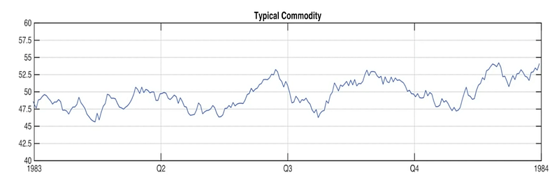
Efficient-market hypothesis¹ states that asset prices reflect all available information. If the hypothesis is true then only insiders with information not available to the public could beat the market and make money solely via trading. In an interview² a mathematician and hedge fund billionaire James Simons strongly disagreed with the hypothesis. He states that there exist patterns in data publicly available that can be used to consistently beat the market. He points out that these patterns come and go. Once people start to abuse certain statistical anomalies, the anomalies vanish. This is because our trades influence the market — especially when there is significant volume involved. An example of a vanished anomaly is the trending of many commodities in the 1980s according to the seasons. One could buy when the price is above a moving average and sell when the price is below it, thus making money each year.
Simon’s argument makes sense — groups of people behave in patterns, and investors are no different. So we can take advantage of people being somewhat predictable with the right mathematical model (which needs to evolve constantly, just like that group of people). Does it mean such a model can make money at no risk and with no limits to the trading volume? Obviously no. The Medallion fund, which is run mostly for fund employees of Renaissance Technologies, is famed for the best track record on Wall Street. The reason why it is mostly for fund employees and not available to every investor is that they had to introduce a capital limit at around 10 billion dollars⁴. At that scale it is very hard not to influence the markets too much, which disrupts the data for the model itself, which in turn makes the predictions incorrect. More and more leading funds have introduced similar capital limits which creates an opportunity for smaller funds to access necessary capital.
On the other hand, the risk cannot be reduced to zero because first, no one knows the exact state of the market (to know the state of the market we would need to know the state of all players, which is impossible) and no one knows exactly how the market will react in the future (butterfly effects of certain actions are possible). Nevertheless, by introducing stochastic variables, which are creations of probability theory, we can model such markets to a certain degree of confidence. The risk cannot be removed but its reduction can be controlled. And because we have stochastic variables in our system, short-term scenarios can vary significantly. Even the best systems can lose money in the short term. For example, in this annual financial report⁵ JP Morgan stated they lose around $100 mln in a single day due to making bad transactions. It’s the long-term result that counts.
Available information: Technical vs Fundamental
Before diving into the models that can use the information to our advantage (that is to reduce investment risks) let us review available information first. Stock exchanges, which record every transaction they mediate, keep their datasets with price and volume data hidden from the public and are willing to sell them only for hundreds of thousands of dollars (usually charged annually). However, cryptocurrency exchanges are much more transparent. Skilled enough programmers should be able to access every transaction ever made on every coin pair (from well-known bitcoin and litecoin to new hot tokens like the recent Reserve Rights Token, RSR) on every major cryptocurrency exchange ‘for free’, not counting time and effort — by using their API. If we assume that the price roughly reflects states of the market we don’t need any other information to make an efficient trading system. However, practice shows such systems can greatly benefit also from analyses of a geopolitical situation/legislative actions/financial reports, etc. (usually referred to as fundamental research). Gold, for example, historically went up in times of emerging conflicts.
Model the market first
Leading quant hedge funds used linear models in the 1980s. Moved on to Hidden Markov Models and later on fully embraced machine learning solutions⁶. No hedge fund brags about their methods but if you keep watching them long enough and you keep attention to details you can find small pieces of information here and there. This is a description of a research scientist position from their website⁷:
Research Scientist: Use machine-learning, applied mathematics, and techniques from modern statistics to develop and refine models of the financial markets and to develop trading algorithms based on those models.
This might seem unimportant at first but pay close attention to this part: “develop and refine models […] and to develop trading algorithms based on those models”. They made a clear distinction between models of the market and trading algorithms. Throughout my research, I also realised that currently, this might be the most efficient way of building a trading system. First — try to model a market. Try to predict certain market states, certain variables, behaviours and only, later on, build a trading algorithm based on your predictions. If you develop a black box that simply takes raw price data and produces trading decisions without intermediate steps it will be much harder to understand and thus modify. And believe me — you will have to modify your first system because no one does it right at the first try. Also, remember that to maintain a trading system one has to modify it periodically which was a conclusion of the previous section (according to Howard Morgan, one of the original team members at Renaissance Technologies, updates their systems monthly⁸).
Feature engineering
If you follow a rule that long term decisions should be driven by long term patterns and short term decisions should be driven mostly by short term pattern — the shorter the time investment window the bigger is the pattern dataset. If we go really short term (sub-seconds or even milliseconds) then the models tend to work better (due to enormous amounts of available data points), however, this leads to expensive computer infrastructure able to make calculations and execute orders very precisely. Since I started my financial journey not by joining one of the existing companies but creating my own, I am personally focused on the minute-to-minute time window, simple due to the technical limitations of a team of 4.
If we extract a data point from each minute (a data point can be a list of numbers such as buy/sell volume, average price weighted by volume in a given minute, minimal price, maximal price, etc.) then we are left with around 500k data points per year. In comparison, during my work on analyses at CERN, we used to make neural network models based on hundreds of millions of data points. Back then we could afford to feed in raw data but in the case of a minute to minute prices they have to be properly simplified to avoid unnecessary overfitting — making models that won’t work properly on unseen data. The spatial representation of these data points might greatly influence the performance. For example — to represent audio it’s much easier to look at the frequencies. If something in the financial world works then it is unlikely that people would share all of the details with others — if you want to be successful you need to be creative and find an appropriate space representation (so-called feature engineering).
Avoiding bias and overfitting
Although it is possible to reliably test the model’s performance on a whole dataset using solutions like k-fold cross-validation, it is often a source of look-ahead bias in many existing articles. For the sake of transparency, I divided bitcoin prices to two datasets: train and test (unseen data for both the algorithm and me). No data after 01.10.2019 was used to train/fit parameters to the model whose results I am going to present. At CERN there is a rule that all physics analyses are first prepared on the previous year’s dataset and no researcher (with very few exceptions) has access to the latest data. This rule was established to prevent all sorts of biases. For example, we know that the price goes down in the test dataset so (maybe only subconsciously) we make a model be more risk aversive. In my work, I also followed this rule and for the most part, I did not look at the latest data (from 01.10.2019 onwards) before this model was built. The model is currently connected to a real exchange trading for me and my clients — this kind of data by definition is free of any kind of bias and I will present some pieces of it to back the simulation.
One of the things one can do to avoid overfitting is introducing a 2-value random variable ‘x’ which allows orders to go into the simulation if ‘x=1’ and block the orders ‘if x=0’. Not having a variable like this in your strategy is equivalent to having it with a mean value of 1. One should try setting the mean value to 0.1 or 0.5 and see what happens with a performance. It’s a real killer of overfitted strategies and/or those with not enough trades to be statistically significant. Let’s introduce the performance ratio R(x) as follows:
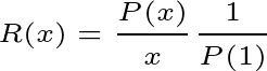
Where P(x) is a performance in a function of x. A robust system should have R(x) constant and around 1.
Simulating realistic transaction fees
The essential feature of any realistic model of a market are transaction fees. Besides paying a commission fee to an exchange we also have to take into account ‘delay fees’, also called slippage. We can never buy/sell using the last seen transaction price. There is always a reaction time of an infrastructure to compute predictions and execute orders. Last but not least, there is a ‘spread fee’ — the difference between ask and bids at a certain order-book depth (especially important in case of trading huge volumes). To conclude, the final fee (FF) is: FF = transaction fee (TF), delay fee (DF), spread fee (SF).
Results
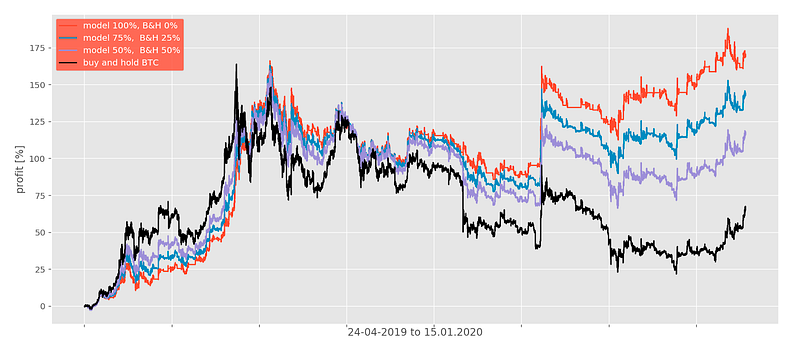
Simulation results for the period 24.04.2019 to 15.01.2020 with different final fees are shown below.
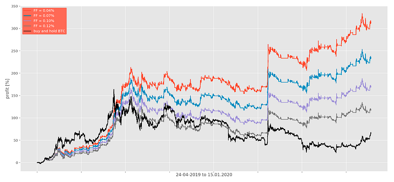
HitBTC offers (taker/maker) 0.07% transaction fees (if you are a verified user) without any additional trading volume requirements. Similarly, Binance offers 0.075% (if you hold BNB but most of its users do). Our system executes a transaction within seconds and the delay fee is around 0.015% on average (if your strategy is a contrarian one, this can be much lower or even negative). The spread fee is around 0.01% for a small investor. SF increases with capital but transaction fees decrease with trading volume, thus making FF relatively constant in terms of capital at around 0.095%. As you can see, this is within a profitable limit.
This level of risk reduction can only be done via active trading on crypto markets. All of the major coins are heavily correlated (from 0.4 to 0.9) so standard methods of risk reductions like asset diversification and rebalancing do not work well⁹.
How to include fundamental input and diversify
If you conduct fundamental research which results suggest the market will go up or down there is a way to increase or decrease the correlation of a strategy with the market.
Let’s say our metric ‘m’ is:

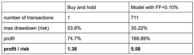
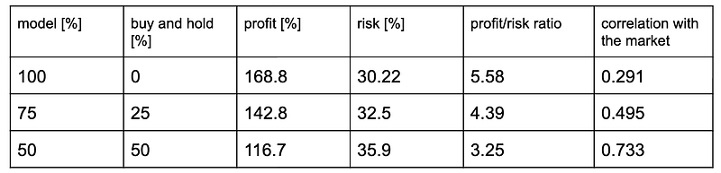
For n=1 we have a balanced strategy where the risk is as important as profit. If we set n<1 we will make our strategy riskier, thus indirectly increasing the correlation with the market. Similarly, n>1 will decrease the correlation. Another method, a more straightforward way to force correlation/decorrelation is diversifying our portfolio in terms of strategies. Instead of putting all our capital into the model we can hold a percentage in the market’s assets or withdraw it from investing. See the plot and table below for comparison.
What’s next?
Since I am collecting more and more data daily, I will further increase the resolution of the decision making up to 4 predictions/decisions in 1 minute in March 2020. This will make the model more sensitive to more rapid movements which are very frequent in 2020 so far.
Note from Towards Data Science’s editors: While we allow independent authors to publish articles in accordance with our rules and guidelines, we do not endorse each author’s contribution. You should not rely on an author’s works without seeking professional advice. See our Reader Terms for details.
Sources:
[1] investopedia
[2] interview available online
[3] interview available online
[4] financial review
[6] Gregory Zuckerman, The Man Who Solved the Market (2019)
[7] rentec website
[8] interview available online