
M2M Day 185: My attempt to intuitively explain how this self-driving car algorithm works
This post is part of Month to Master, a 12-month accelerated learning project. For May, my goal is to build the software part of a self-driving car.
Yesterday, I figured out how to identify lane lines in a forward-facing image of the road. Well… I at least figured out how to run code that could do this.
Truthfully, I didn’t understand how the code actually worked, so today I tried to change that.
Below is the main block of code I used yesterday. In particular, I’ve copied the primary function, which is called “draw_lane_lines”. Basically, a function is a block of code that takes some input (in this case a photo), manipulates the input in some way, and then outputs the manipulation (in this case the lane lines).
This primary function uses some other helper functions defined elsewhere in the code, but these helper functions are mostly just slightly cleaner ways of consuming the pre-made functions from the libraries I downloaded yesterday (like OpenCV, for example).
def draw_lane_lines(image): imshape = image.shape
# Greyscale image
greyscaled_image = grayscale(image)
# Gaussian Blur
blurred_grey_image = gaussian_blur(greyscaled_image, 5)
# Canny edge detection
edges_image = canny(blurred_grey_image, 50, 150)
# Mask edges image
border = 0
vertices = np.array([[(0,imshape[0]),(465, 320), (475, 320),
(imshape[1],imshape[0])]], dtype=np.int32)
edges_image_with_mask = region_of_interest(edges_image,
vertices)
# Hough lines
rho = 2
theta = np.pi/180
threshold = 45
min_line_len = 40
max_line_gap = 100
lines_image = hough_lines(edges_image_with_mask, rho, theta,
threshold, min_line_len, max_line_gap) # Convert Hough from single channel to RGB to prep for weighted
hough_rgb_image = cv2.cvtColor(lines_image, cv2.COLOR_GRAY2BGR)
# Combine lines image with original image
final_image = weighted_img(hough_rgb_image, image)
return final_imageThe bolded comments are descriptions of the main parts of the image processing pipeline, which basically means these are the seven manipulations performed sequentially on the input image in order to output the lane lines.
Today, my goal was to understand what each of these seven steps did and why they were being used.
Actually, I only focused on the first five, which output the mathematical representation of the lane lines. The last two manipulations just create the visuals so us humans can visually appreciate the math (in other words, these steps aren’t necessary when a self-driving car is actually consuming the outputted data).
Thus, based on my research today, I will now attempt to explain the following sequence of image processing events: Input image → 1. Greyscale image, 2. Gaussian Blur, 3. Canny edge detection, 4. Mask edges image, 5. Hough lines → Lane line output
Input image
Here’s the starting input image.
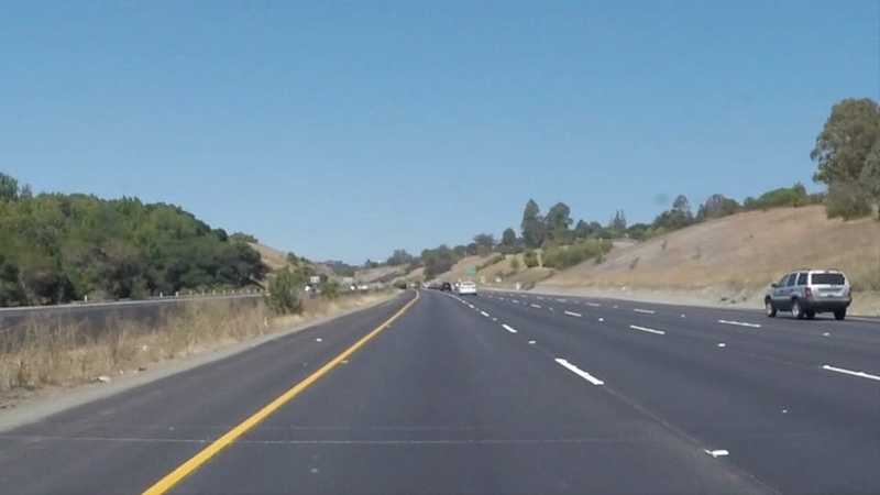
It’s important to remember that an image is nothing more than a bunch of pixels arranged in a rectangle. This particular rectangle is 960 pixels by 540 pixels.
The value of each pixel is some combination of red, green, and blue, and is represented by a triplet of numbers, where each number corresponds to the value of one of the colors. The value of each of the colors can range from 0 to 255, where 0 is the complete absence of the color and 255 is 100% intensity.
For example, the color white is represented as (255, 255, 255) and the color black is represented as (0, 0, 0).
So, this input image can be described by 960 x 540 = 518,400 triplets of numbers ranging from (0, 0, 0) to (255, 255, 255).
Now that this image is just a collection of numbers, we can start manipulating these numbers in useful ways using math.
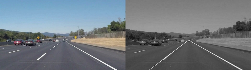
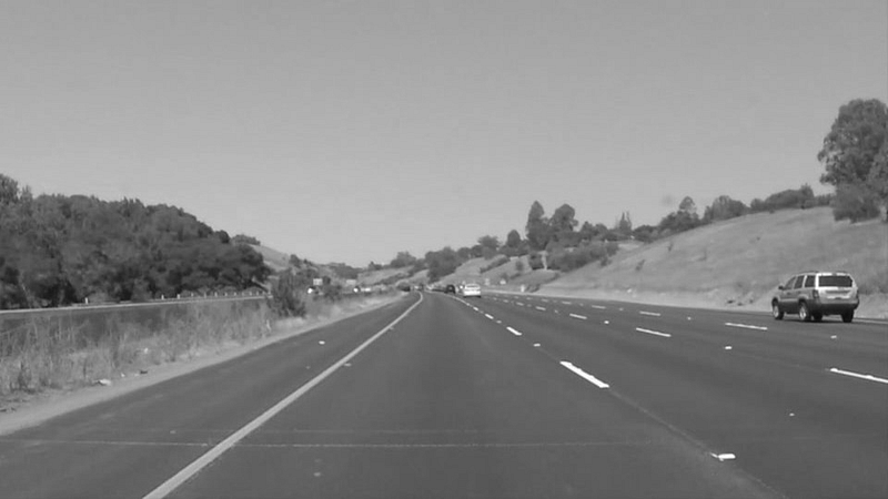
1. Greyscale image
The first processing step is to convert the the color image to greyscale, effectively downgrading the color space from three-dimensions to one-dimension. It’s much easier (and more effective) to manipulate the image in only one-dimension: This one dimension is the “darkness” or “intensity” of the pixel, with 0 representing black, 255 representing white, and 126 representing some middle grey color.
Intuitively, I expected that a greyscale filter would just be a function that averaged the red, blue, and green values together to arrive at the greyscale output.
So for example, here’s a color from the sky in the original photo:

It can be represented in RGB (red, green, blue) space as (120, 172, 209).
If I average these values together I get (120 + 172 + 209)/3 = 167, or this color in greyscale space.

But, it turns out, when I convert this color to greyscale using the above function, the actual outputted color is 164, which is slightly different than what I generated using my simple averaging method.

While my method isn’t actually “wrong” per se, the common method used is to compute a weighted average that better matches how our eyes perceive color. In other words, since our eyes have many more green receptors than red or blue receptors, the value for green should be weighted more heavily in the greyscale function.
One common method, called colometric conversion uses this weighted sum: 0.2126 Red + 0.7152 Green + 0.0722 Blue.
After processing the original image through the greyscale filter, we get this output…
2. Gaussian Blur
The next step is to blur the image using a Gaussian Blur.
By applying a slight blur, we can remove the highest-frequency information (a.k.a noise) from the image, which will give us “smoother” blocks of color that we can analyze.
Once again, the underlying math of a Gaussian Blur is very basic: A blur just takes more averages of pixels (this averaging process is a type of kernel convolution, which is an unnecessarily fancy name for what I’m about to explain).
Basically, to generate a blur, you must complete the following steps:
- Select a pixel in the photo and determine it’s value
- Find the values for the selected pixel’s local neighbors (we can arbitrarily define the size of this “local region”, but it’s typically fairly small)
- Take the value of the original pixel and the neighbor pixels and average them together using some weighting system
- Replace the value of the original pixel with the outputted averaged value
- Do this for all pixels
This process is essentially saying “make all the pixels more similar to the pixels nearby”, which intuitively sounds like blurring.
For a Gaussian Blur, we are simply using the Gaussian Distribution (i.e. a bell curve) to determine the weights in Step 3 above. This means that the closer a pixel is to the selected pixel, the greater its weight.
Anyway, we don’t want to blur the image too much, but just enough so that we can remove some noise from the photo. Here’s what we get…

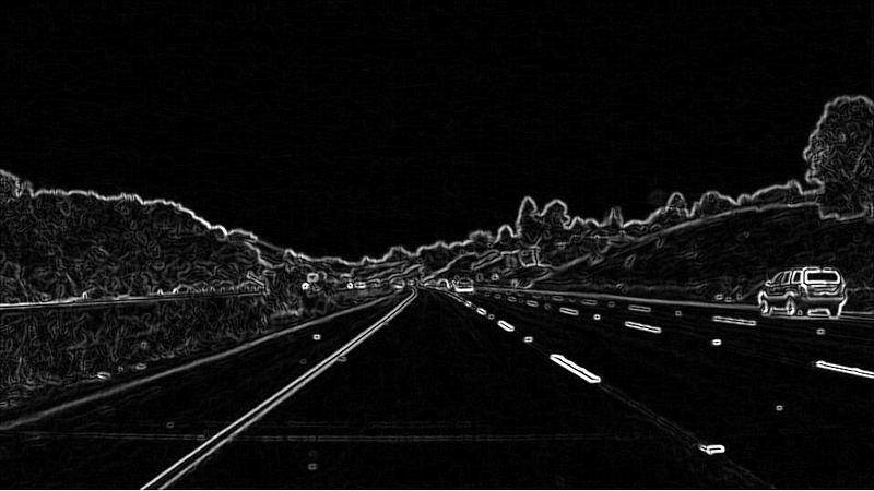
3. Canny edge detection
Now that we have a greyscaled and Gaussian Blurred image, we are going to try to find all the edges in this photo.
An edge is simply an area in the image where there is a sudden jump in value.
For example, there is a clear edge between the grey road and the dashed white line, since the grey road may have a value of something like 126, the white line has a value close to 255, and there is no gradual transition between these values.
Again, the Canny Edge Detection filter uses very simple math to find edges:
- Select a pixel in the photo
- Identify the value for the group of pixels to the left and the group of pixels to the right of the selected pixel
- Take the difference between these two groups (i.e. subtract the value of one from the other).
- Change the value of the selected pixel to the value of the difference computed in Step 3.
- Do this for all pixels.
So, pretend that we are only looking at the one pixel to the left and to the right of the selected pixel, and imagine these are the values: (Left pixel, selected pixel, right pixel) = (133, 134, 155). Then, we would compute the difference between the right and left pixel, 155–133 = 22, and set the new value of the selected pixel to 22.
If the selected pixel is an edge, the difference between the left and right pixels will be a greater number (closer to 255) and therefore will show up as white in the outputted image. If the selected pixel isn’t an edge, the difference will be close to 0 and will show up as black.
Of course, you may have noticed that the above method would only find edges in the vertical direction, so we must do a second process where we compare the pixels above and below the selected pixel to address edges in the horizontal direction.
These differences are called gradients, and we can compute the total gradient by essentially using the Pythagorean Theorem to add up the individual contributions from the vertical and horizontal gradients. In other words, we can say that the total gradient²= the vertical gradient²+ the horizontal gradient².
So, for example, let’s say the vertical gradient = 22 and the horizontal gradient = 143, then the total gradient = sqrt(22²+143²) = ~145.
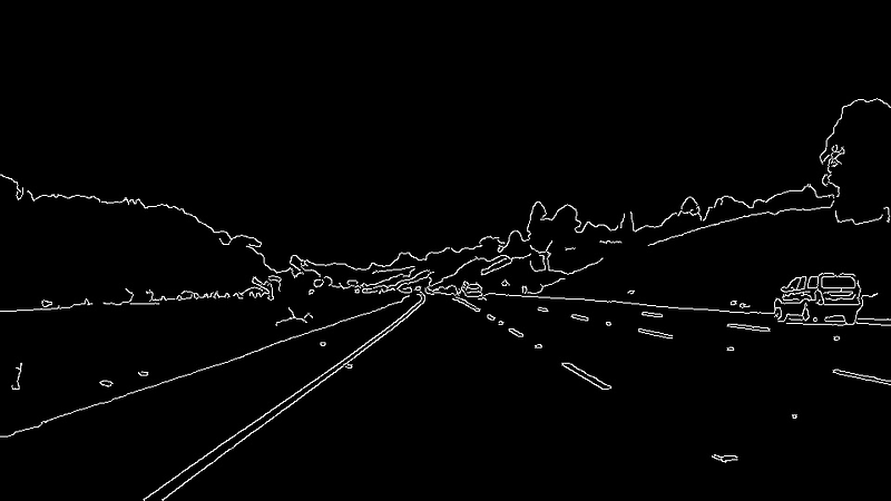
The output looks something like this…
The Canny Edge Detection filter now completes one more step.
Rather than just showing all edges, the Canny Edge Detection filter tries to identify the important edges.
To do this, we set two thresholds: A high threshold and a low threshold. Let’s say the high threshold is 200 and the low threshold is 150.
For any total gradient that has a value greater than the high threshold of 200, that pixel automatically is considered an edge and is converted to pure white (255). For any total gradient that has a value less than the low threshold of 155, that pixel automatically is considered “not an edge” and is converted to pure black (0).
For any gradient in between 150 and 200, the pixel is counted as an edge only if it is directly touching another pixel that has already been counted as an edge.
The assumption here is that if this soft edge is connected to the hard edge, it is probably part of the same object.
After completing this process for all pixels, we get an image that looks like this…
4. Mask edges image
This next step is very simple: A mask is created that eliminates all parts of the photo we assume not to have lane lines.
We get this…
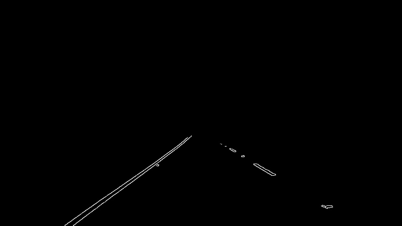
It seems like this a pretty aggressive and presumptuous mask, but this is what is currently written in the original code. So, moving on…
5. Hough lines
The final step is to use the Hough transform to find the mathematical expression for the lane lines.
The math behind the Hough transform is slightly more complicated than all the weighted average stuff we did above, but only barely.
Here’s the basic concept:
The equation for a line is y = mx + b, where m and b are constants that represent the slope of the line and the y-intercept of the line respectively.
Essentially, to use the Hough transform, we determine some 2-dimensional space of m’s and b’s. This space represents all the combinations of m’s and b’s we think could possible generate the best-fitting line for the lane lines.
Then, we navigate through this space of m’s and b’s, and for each pair (m,b), we can determine an equation for a particular line of the form y = mx + b. At this point, we want to test this line, so we find all the pixels that lie on this line in the photo and ask them to vote if this is a good guess for the lane line or not. The pixel votes “yes” if it’s white (a.k.a part of an edge) and votes “no” if it’s black.
The (m,b) pair that gets the most votes (or in this case, the two pairs that get the most votes) are determined to be the two lane lines.
Here’s the output of the Hough Transform…
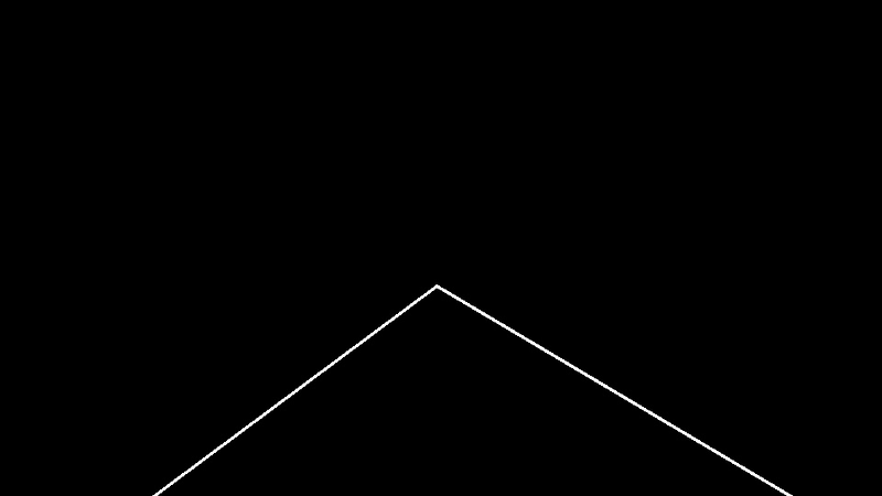
I’m skipping over the part where, rather than using the formula y = mx + b to represent the line, the Hough transform instead uses a polar coordinates- / trigonometric- style representation that uses rho and theta as the two parameters.
This distinction isn’t super important (for our understanding), since the space is still being parametrized in 2-dimensions, and the logic is exactly the same, but this trigonometric representation does help with the fact that we can’t express completely vertical lines with the y = mx + b equation.
Anyway, this is why rho and theta are being used in the above code.
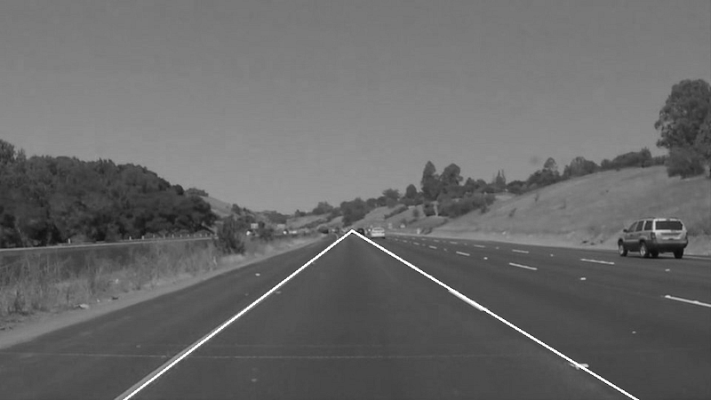
The Final Output
And we are done.
The program outputs the two parameters to describe the two lane lines (interestingly, these outputs are converted back to the m, b parametrization). The program also provides the coordinates of each lane line’s end points.
Lane line 1
Slope: -0.740605727717; Intercept: 664.075746144
Point one: (475, 311) Point two: (960, 599)
Lane line 2
Coef: -0.740605727717; Intercept: 664.075746144
Point one: (475, 311) Point two: (0, 664)
Overlaying these lines on the original image, we see that we’ve effectively identified the lane lines, using basic math operations.
Read the next post. Read the previous post.