Time-Series Forecasting: Predicting Stock Prices Using An LSTM Model

In this post I show you how to predict stock prices using a forecasting LSTM model

1. Introduction

1.1. Time-series & forecasting models

Traditionally most machine learning (ML) models use as input features some observations (samples / examples) but there is no time dimension in the data.

Time-series forecasting models are the models that are capable to predict future values based on previously observed values. Time-series forecasting is widely used for non-stationary data. Non-stationary data are called the data whose statistical properties e.g. the mean and standard deviation are not constant over time but instead, these metrics vary over time.

These non-stationary input data (used as input to these models) are usually called time-series. Some examples of time-series include the temperature values over time, stock price over time, price of a house over time etc. So, the input is a signal (time-series) that is defined by observations taken sequentially in time.

A time series is a sequence of observations taken sequentially in time.

Observation: Time-series data is recorded on a discrete time scale.

Disclaimer (before we move on): There have been attempts to predict stock prices using time series analysis algorithms, though they still cannot be used to place bets in the real market. This is just a tutorial article that does not intent in any way to “direct” people into buying stocks.

• My mailing list in just 5 seconds: https://seralouk.medium.com/subscribe
• Become a member and support me:https://seralouk.medium.com/membership
• NEW: After a great deal of hard work and staying behind the scenes for quite a while, we’re excited to now offer our expertise through a platform, the “Data Science Hub” on Patreon (https://www.patreon.com/TheDataScienceHub). This hub is our way of providing you with bespoke consulting services and comprehensive responses to all your inquiries, ranging from Machine Learning to strategic data analytics

2. The LSTM model

Long short-term memory (LSTM) is an artificial recurrent neural network (RNN) architecture used in the field of deep learning. Unlike standard feedforward neural networks, LSTM has feedback connections. It can not only process single data points (e.g. images), but also entire sequences of data (such as speech or video inputs).

LSTM models are able to store information over a period of time.

In order words, they have a memory capacity. Remember that LSTM stands for Long Short-Term Memory Model.

This characteristic is extremely useful when we deal with Time-Series or Sequential Data. When using an LSTM model we are free and able to decide what information will be stored and what discarded. We do that using the “gates”. The deep understanding of the LSTM is outside the scope of this post but if you are interested in learning more, have a look at the references at the end of this post.

If you want to learn Data Science by yourself with the support of interactive roadmaps and an active learning community have a look at this resource: https://aigents.co/learn

3. Getting the stock price history data

Thanks to Yahoo finance we can get the data for free. Use the following link to get the stock price history of TESLA: https://finance.yahoo.com/quote/TSLA/history?period1=1436486400&period2=1594339200&interval=1d&filter=history&frequency=1d

You should see the following:

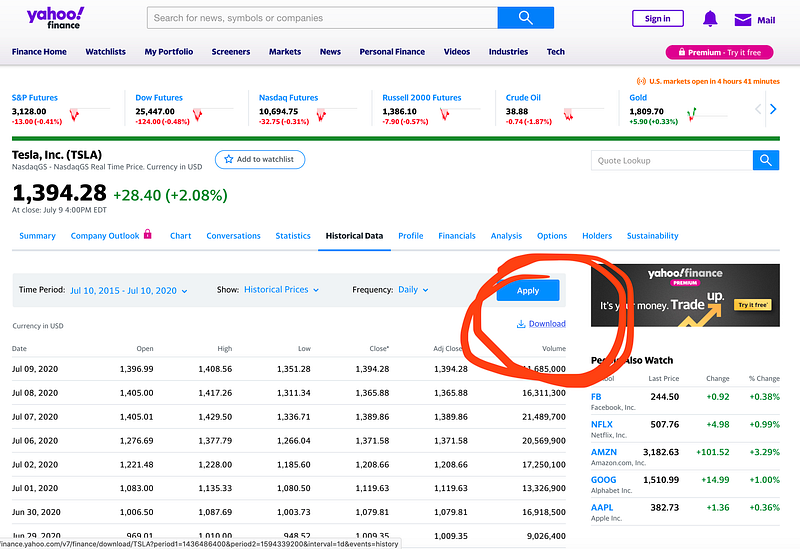
Click on the Download and save the .csv file locally on your computer.

The data are from 2015 till now (2020) !

4.Python working example

Modules needed: Keras, Tensorflow, Pandas, Scikit-Learn & Numpy

We are going to build a multi-layer LSTM recurrent neural network to predict the last value of a sequence of values i.e. the TESLA stock price in this example.

Let’s load the data and inspect them:

import math
import matplotlib.pyplot as plt
import keras
import pandas as pd
import numpy as np
from keras.models import Sequential
from keras.layers import Dense
from keras.layers import LSTM
from keras.layers import Dropout
from keras.layers import *
from sklearn.preprocessing import MinMaxScaler
from sklearn.metrics import mean_squared_error
from sklearn.metrics import mean_absolute_error
from sklearn.model_selection import train_test_split
from keras.callbacks import EarlyStopping

df=pd.read_csv("TSLA.csv")
print(‘Number of rows and columns:’, df.shape)
df.head(5)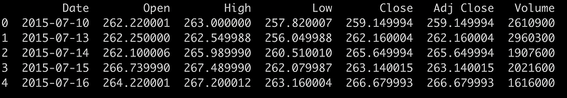

The next step is to split the data into training and test sets to avoid overfitting and to be able to investigate the generalization ability of our model. To learn more about overfitting read this article:

The target value to be predicted is going to be the “Close” stock price value.

training_set = df.iloc[:800, 1:2].values
test_set = df.iloc[800:, 1:2].values

It’s a good idea to normalize the data before model fitting. This will boost the performance. You can read more here for the Min-Max Scaler:

Let’s build the input features with time lag of 1 day (lag 1):

# Feature Scaling
sc = MinMaxScaler(feature_range = (0, 1))
training_set_scaled = sc.fit_transform(training_set)

# Creating a data structure with 60 time-steps and 1 output
X_train = []
y_train = []
for i in range(60, 800):
    X_train.append(training_set_scaled[i-60:i, 0])
    y_train.append(training_set_scaled[i, 0])
X_train, y_train = np.array(X_train), np.array(y_train)

X_train = np.reshape(X_train, (X_train.shape[0], X_train.shape[1], 1))
#(740, 60, 1)

We have now reshaped the data into the following format (#values, #time-steps, #1 dimensional output).

Now, it’s time to build the model. We will build the LSTM with 50 neurons and 4 hidden layers. Finally, we will assign 1 neuron in the output layer for predicting the normalized stock price. We will use the MSE loss function and the Adam stochastic gradient descent optimizer.

Note: the following will take some time (~5min).

model = Sequential()

#Adding the first LSTM layer and some Dropout regularisation
model.add(LSTM(units = 50, return_sequences = True, input_shape = (X_train.shape[1], 1)))
model.add(Dropout(0.2))

# Adding a second LSTM layer and some Dropout regularisation
model.add(LSTM(units = 50, return_sequences = True))
model.add(Dropout(0.2))

# Adding a third LSTM layer and some Dropout regularisation
model.add(LSTM(units = 50, return_sequences = True))
model.add(Dropout(0.2))

# Adding a fourth LSTM layer and some Dropout regularisation
model.add(LSTM(units = 50))
model.add(Dropout(0.2))

# Adding the output layer
model.add(Dense(units = 1))

# Compiling the RNN
model.compile(optimizer = 'adam', loss = 'mean_squared_error')

# Fitting the RNN to the Training set
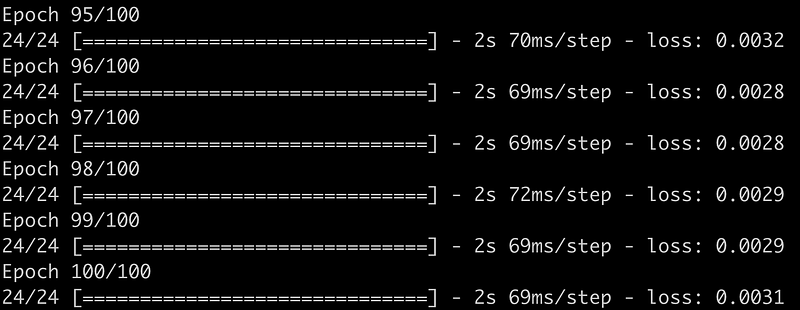
model.fit(X_train, y_train, epochs = 100, batch_size = 32)

When the fitting is finished you should see something like this:

Prepare the test data (reshape them):

# Getting the predicted stock price of 2017
dataset_train = df.iloc[:800, 1:2]
dataset_test = df.iloc[800:, 1:2]

dataset_total = pd.concat((dataset_train, dataset_test), axis = 0)

inputs = dataset_total[len(dataset_total) - len(dataset_test) - 60:].values

inputs = inputs.reshape(-1,1)
inputs = sc.transform(inputs)
X_test = []
for i in range(60, 519):
    X_test.append(inputs[i-60:i, 0])
X_test = np.array(X_test)
X_test = np.reshape(X_test, (X_test.shape[0], X_test.shape[1], 1))

print(X_test.shape)
# (459, 60, 1)

Make Predictions using the test set

predicted_stock_price = model.predict(X_test)
predicted_stock_price = sc.inverse_transform(predicted_stock_price)

Let’s visualize the results now:

# Visualising the results
plt.plot(df.loc[800:, ‘Date’],dataset_test.values, color = ‘red’, label = ‘Real TESLA Stock Price’)
plt.plot(df.loc[800:, ‘Date’],predicted_stock_price, color = ‘blue’, label = ‘Predicted TESLA Stock Price’)
plt.xticks(np.arange(0,459,50))
plt.title('TESLA Stock Price Prediction')
plt.xlabel('Time')
plt.ylabel('TESLA Stock Price')
plt.legend()
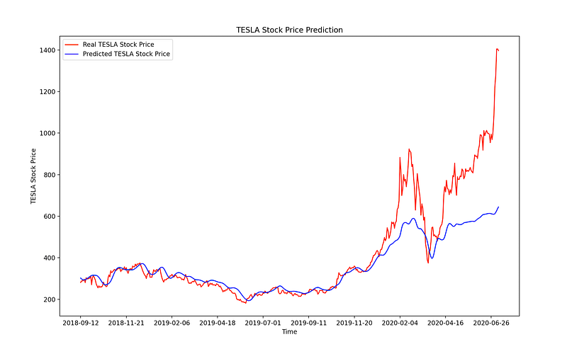
plt.show()

5. Results

Using a lag of 1 (i.e. step of one day):

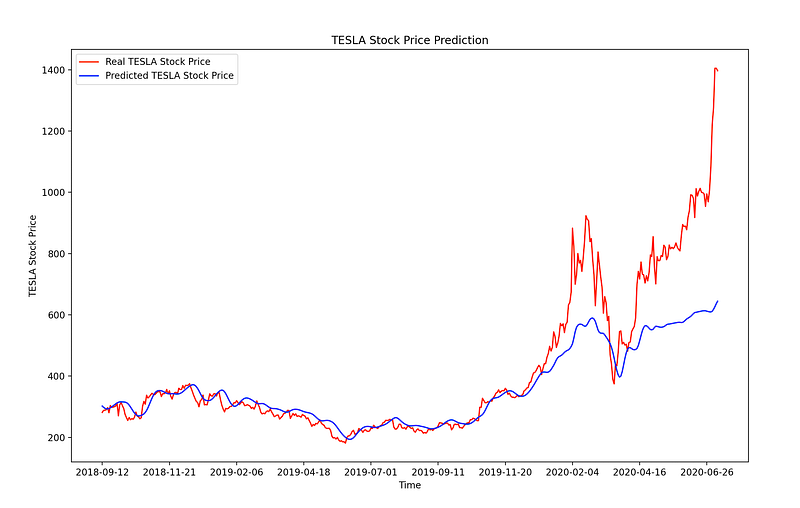
Observation: Huge drop in March 2020 due to the COVID-19 lockdown !

We can clearly see that our model performed very good. It is able to accuretly follow most of the unexcepted jumps/drops however, for the most recent date stamps, we can see that the model expected (predicted) lower values compared to the real values of the stock price.

If you’re passionate about diving deeper into machine learning with Python and sklearn, I highly recommend checking out this book; it’s a game-changer in breaking down complex topics into digestible insights.

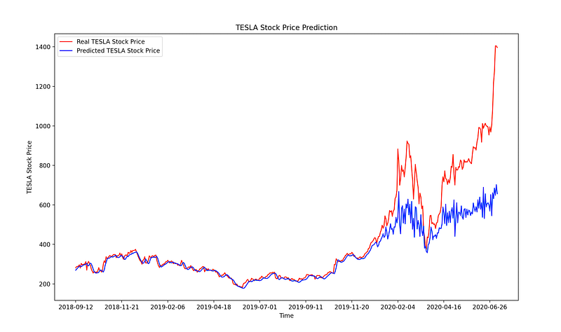
A note about the lag

The initial selected lag in this article was 1 i.e. using a step of 1 day. This can be easily changed by altering the code that builds the 3D inputs.

Example: One can change the following 2 blocks of code:

X_train = []
y_train = []
for i in range(60, 800):
    X_train.append(training_set_scaled[i-60:i, 0])
    y_train.append(training_set_scaled[i, 0])

and

X_test = []
y_test = []
for i in range(60, 519):
    X_test.append(inputs[i-60:i, 0])
X_test = np.array(X_test)
X_test = np.reshape(X_test, (X_test.shape[0], X_test.shape[1], 1))

with the following new code:

X_train = []
y_train = []
for i in range(60, 800):
    X_train.append(training_set_scaled[i-50:i, 0])
    y_train.append(training_set_scaled[i, 0])

and

X_test = []
y_test = []
for i in range(60, 519):
    X_test.append(inputs[i-50:i, 0])
X_test = np.array(X_test)
X_test = np.reshape(X_test, (X_test.shape[0], X_test.shape[1], 1))

In that case the results look like this:

That’s all folks ! Hope you liked this article!

• NEW: After a great deal of hard work and staying behind the scenes for quite a while, we’re excited to now offer our expertise through a platform, the “Data Science Hub” on Patreon (https://www.patreon.com/TheDataScienceHub). This hub is our way of providing you with bespoke consulting services and comprehensive responses to all your inquiries, ranging from Machine Learning to strategic data analytics planning.
• Another resource. Learn Data Science and ML with the help of an 🤖 AI-powered tutor. Start here https://aigents.co/learn choose a topic and he will show up where you need him. No paywall, no signups, no ads.

More readings:

Have a look at my Facebook Prophet model that I used to predict the GOOGLE stock price in another article.

Check also my recent article using an ARIMA model:

References

[1] https://colah.github.io/posts/2015-08-Understanding-LSTMs/

[2] https://en.wikipedia.org/wiki/Long_short-term_memory

Stay tuned & support this effort

If you liked and found this article useful, follow me to be able to see all my new posts.

Questions? Post them as a comment and I will reply as soon as possible.

Latest posts

Get in touch with me

• LinkedIn: https://www.linkedin.com/in/serafeim-loukas/
• ResearchGate: https://www.researchgate.net/profile/Serafeim_Loukas
• EPFL profile: https://people.epfl.ch/serafeim.loukas
• Stack Overflow: https://stackoverflow.com/users/5025009/seralouk