
LSTM Model Trying To Predict Future Price Movement
Coding a LSTM model from scratch to predict future price movements.
Part 1: Setting Up Colab
#import libraries
from pandas_datareader import data
import matplotlib.pyplot as plt
import pandas as pd
import datetime as dt
import urllib.request, json
import os
import numpy as np
import tensorflow as tf
from sklearn.preprocessing import MinMaxScaler
This code includes several libraries and modules that are essential for analyzing and visualizing data, as well as for machine learning. The first library, pandas_datareader, allows us to collect financial information from various sources. The next library, matplotlib.pyplot, allows us to create visually appealing charts and graphs. Another library, pandas, helps with analyzing and manipulating data. The library datetime comes in handy when working with dates and times. To make HTTP requests, the library urllib.request is used. When dealing with JSON data, the library json is helpful. The library os allows us to interact with our operating system. For scientific calculations, the library numpy is used. For machine learning tasks, the library tensorflow is utilized. Finally, the library MinMaxScaler helps us scale data to prepare for machine learning models. All these libraries are imported so that we can effectively perform a variety of data analysis and machine learning tasks.
#declare name of your device and drive location select GPU
device_name = tf.test.gpu_device_name()
if device_name != '/device:GPU:0':
  raise SystemError('GPU device not found')
print('Found GPU at: {}'.format(device_name))
This piece of code sets the name for the device and chooses where it will be stored. It then double checks to make sure the name for the graphics card is correct, and if it isnt, it will display an error message. Once that is done, it will let you know that a graphics card has been found at the chosen location.
So here this time, I was thinking about using general electric dataset instead of usual amazon.
This new dataset is larger and it’s easier to observe their progress for longer time than amzn. If I need 900 data samples for training all I have to run testing on 180 days, but the rise of amazon has been around for 4 years to this date, so the data is limited especially for this kind of one day prediction and detecting price pattern.
This new dataset is larger this time and so I don’t have to worry about overfitting and I can focus more on training.
#Get your API data
df = pd.read_csv(os.path.join(f'{googlepath}','ge.us.txt'),delimiter=',',usecols=['Date','Open','High','Low','Close'])
This program helps us get important information from a website. The df variable is what we will use to store this information in a neat and organized way. To start, we bring in the pandas library using the shortcut pd. This library is often used to analyze and work with data in Python. Our next step is to use the read_csv function from pandas, which lets us take data from a CSV file. When using this function, we have to specify two things: where the file is located, and how the data is separated. We do this using os.path.join, which combines the googlepath and ge.us.txt variables to create a file path, and by saying that the data is split by commas. Finally, we tell the program which parts of the CSV file we want to keep, which in this case are the columns with the Date, Open, High, Low, and Close information. The data is then saved in the df variable so that we can use it later for more analyzing and organizing.
Find Average Price of High and Low Prices And Use That To Plot
plt.figure(figsize = (18,9))
plt.plot(range(df.shape[0]),(df['Low']+df['High'])/2.0)
plt.xticks(range(0,df.shape[0],500),df['Date'].loc[::500],rotation=45)
plt.xlabel('Date',fontsize=18)
plt.ylabel('avg Price',fontsize=18)
plt.show()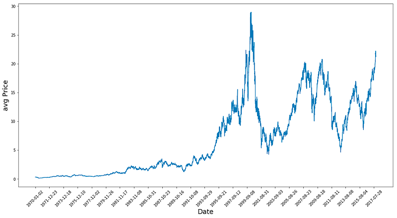
This program first makes a new picture with a size of 18 by 9 using the plt.figure function. Then, it draws a line graph by finding the average of the Low and High numbers for each row in the table. To make it easier to read, the plt.xticks function is used to show only every 500th date from the Date column. The labels for the x-axis and y-axis are also made bigger, with a font size of 18. To improve the look, the label text is tilted at a 45 degree angle. Finally, the graph is shown using the plt.show function.
# First calculate the average prices from the highest and lowest
high_prices = df.loc[:,'High'].as_matrix()
low_prices = df.loc[:,'Low'].as_matrix()
avg_prices = (high_prices+low_prices)/2.0
This program is finding the middle price from a set of data. It first looks for the column labeled High and puts that information into a collection called high_prices. Then, it does the same thing for the column labeled Low and stores that in a collection called low_prices. Next, the program adds up the numbers in both collections and divides them by 2 to get the average price. This average is then saved in a variable called avg_prices for future use. This process is repeated for each row of data, giving us an average price for each row.
Observations
- Data Peaks around 1983 and then grows until the 2 crashes.
- Calculating average prices Is somehow normalising the data and giving a much better picture than using only high prices or closing prices since it gives an idea about business around.
train = avg_prices[:11000]
test = avg_prices[11000:]
len(avg_prices)
This code generates two fresh variables, train and test, which hold distinct components of another variable called avg_prices. The train variable comprises of the first 11000 elements from the avg_prices variable, while the test variable includes all the remaining elements. Later, the length of the avg_prices list is determined, which tells us the total number of items in it.
Start Normalising Data
scaler = MinMaxScaler() #use mimaxscaler from scikitlearn to normalize data
train = train.reshape(-1,1)
test = test.reshape(-1,1)
This code uses the MinMaxScaler function from the scikitlearn library to make sure the data is in a consistent format. First, the function is given the nickname scaler. Then, the information from the train and test datasets is adjusted so it only has one column, which makes it easier for the scaler to work with. The scaler function then uses this data to change the values so they all fall between 0 and 1. This is helpful when dealing with different datasets that have different value ranges because it makes sure all the data is on the same scale. Normalizing also helps when there are different units of measurement.
Normalise average prices and trying to predict based on them instead of feature generation length of data is 12075.
window_size = 2500
for x in range(0,10000,window_size):
    scaler.fit(train[x:x+window_size,:])
    train[x:x+window_size,:] = scaler.transform(train[x:x+window_size,:])

scaler.fit(train[x+window_size:,:])
train[x+window_size:,:] = scaler.transform(train[x+window_size:,:])
First, we set a variable called window_size and give it the number 2500. This variable will help us make separate groups of data that dont overlap. Then, we use a for loop to go through numbers from 0 to 10000, with each group being 2500 numbers apart. This gives us groups of data that are each 2500 numbers long. Inside the loop, we use a scaler tool to adjust and change a part of the training data. The scaler tool takes the average and standard deviation of the data in each group. Then, it changes the data by subtracting the average and dividing by the standard deviation for each column. We put this new, changed data back in the same place as the original data, replacing it. The loop goes through this process for each group of data until it has gone through all of the training data. This makes sure that we change all of the data, not just one group. In the last part of the code, we use the scaler again to change any remaining data in the training set that wasnt included in the previous groups. This means now all of the data has been changed the same way and is ready for us to do more with it.
# Reshape both train and test data
train = train.reshape(-1)
First, the code takes the variable train and applies the reshape method to it, using the argument -1. This modifies the arrangement of the information stored in the variable. By using -1 as the argument, the code can determine the appropriate arrangement without needing specific instructions, since it depends on the amount of information present. This is particularly helpful when dealing with datasets of different sizes. As a result, the variables content is changed for both the train and test data, making them easier to handle and compare for future data examination.
Making this into a 2d shape train
# Normalize test data
test = scaler.transform(test).reshape(-1)
This piece of code works with a variable named test that supposedly holds some information. Next, it makes use of a method known as transform from an object referred to as scaler to alter the data in test. From what is understood, this scaler object helps make the data more uniform in some way, but the exact steps of this process are not specified. Once the alteration is complete, the outcome is reconfigured into a one-dimensional form using another method called reshape and then saved back into the variable test. This makes it easier to examine or carry out any additional actions on the standardized data.
EMA Averaging
EMA = 0.0 # keep EMA 0.0
ema2 = 0.1 # gamma is a variabe that can be multiplied with train
for i in range(11000):
  EMA = ema2*train[i] + (1-ema2)*EMA
  train[i] = EMA
In this code, we are setting up EMA and ema2, which are used to calculate an exponentially weighted average. We are starting with a certain set of values for EMA and ema2. Then, with a for loop, we are going through each element in train represented by i and calculating a new value for EMA. This new value takes into account the original value of EMA, as well as the value of gamma, which we can adjust. After each calculation, the loop continues to the next element, updating the overall EMA as it goes. Finally, we update the train array with the new EMA values, giving us a complete array of updated averages for the original data.
# Used for visualization and test purposes
all_avg_data = np.concatenate([train,test],axis=0)
This code helps combine two arrays, train and test, and create a new array called all_avg_data. The function used for this is concatenate, and it comes from the numpy library, which is used for doing math and science in Python. The goal of making this new array is to examine and experiment with something, possibly information or data from the original arrays. The axis=0 determines that the two arrays will be combined in the first row, so the new array will have the same columns as the original arrays combined. This code doesnt show any results, it simply makes a new array with the merged data for later use.
One Step Ahead Predictions Via Averaging
window_size = 100 # chose standard window size of 100
N = train.size
mse_err = []
_avg_pred = [] #create a list for average x, predictions and mse errors
_avg_x = []

for idx1 in range(window_size,N): #make a for loop where if the value is greater than size then use timedelta function for that 1 day

    if idx1 >= N:
        date = dt.datetime.strptime(k, '%Y-%m-%d').date() + dt.timedelta(days=1)
    else:
        date = df.loc[idx1,'Date']  #if not just find that value in the dataframe for the data and put it in date

    _avg_pred.append(np.mean(train[idx1-window_size:idx1])) #Keep apending values into into the lists
    mse_err.append((_avg_pred[-1]-train[idx1])**2)   #calculate mse errors
    _avg_x.append(date) #this is the x train for averages we will use to train

print('MSE error for standard averaging: %.5f'%(0.5*np.mean(mse_err)))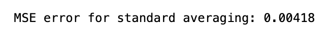
This piece of code is designed to figure out Mean Square Error MSE for a machine learning program. The first line determines a window size of 100. Then, the variable N is set to represent the number of data points in the training dataset. Next, three lists are made to hold the average x values, predictions, and MSE errors. The for loop goes through each data point in the training set, starting from the window size and going all the way to the end. During each iteration, it checks if the current index is the same or higher than the total number of data points. If it is, it uses the timedelta function to add one day to the current date. If not, it assigns the current dates value to the date variable. The next line adds the average of the previous data points to the avg_pred list. Then it calculates the MSE error by taking the difference between the current average prediction and the actual value, squaring it, and adding it to the mse_err list. Finally, the loop adds the current date to the avg_x list. As a final step, the code shows the MSE error, calculated through the standard averaging formula, which multiplies the average of squared errors by 0.5. Ultimately, this code measures MSE for a machine learning program using a window size of 100.
for range from 100 to size of train(11000) create the training data dates and then find their mean and append them to average predictions
else:
make a test set and then append all this to std_avg(all dates in this)
and:
calculate the mse_err
The above method is super awesome to calculate simple or standard averages. It uses timedelta to mainpulate date and push the date back to 1 day and add it to date along with datetime which strups the date and time from the given format.
plt.figure(figsize = (18,9))
plt.plot(range(df.shape[0]),all_avg_data,color='y',label='True')
plt.plot(range(window_size,N),_avg_pred,color='b',label='Prediction')
plt.xlabel('Date')
plt.ylabel('avg Price')
plt.legend(fontsize=18)
plt.show()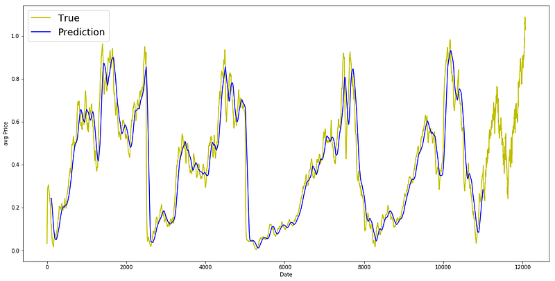
this code helps us see and compare the actual and predicted average data on a graph.
Everythign worked, Now let’s exponential moving average similar to what we tried in previous articles.
window_size = 100
N = train.size
mse_err = []
_avg_predictions_run = []
_avg_x_run = []


running_mean = 0.0 #the mean tat is calculates
_avg_predictions_run.append(running_mean)

decay = 0.5 # use this to average the running mean again;

for idx1 in range(1,N): #range from 1 to N-1

    running_mean = running_mean*decay + (1.0-decay)*train[idx1-1] #the remaining prob multiplied by the train sets data points
    _avg_predictions_run.append(running_mean)
    mse_err.append((_avg_predictions_run[-1]-train[idx1])**2) #make mse error with the help of train set
    _avg_x_run.append(date) #append the dates into the list

print('MSE error for EMA averaging: %.5f'%(0.5*np.mean(mse_err))) #Calculate MSE
The following code calculates the average and MSE Mean Squared Error values for a group of data points. First, it sets the window size to 100, which will be used in the calculation. Then, it determines the size of the training set and creates empty lists to store the MSE error, average predictions, and average x values. The initial running mean is set to 0.0 and stored in the list _avg_predictions. The decay value is then set to 0.5, which is used in the calculation of the average running mean. The code then loops through the training set from index 1 to N-1. Within the loop, the running mean is multiplied by the decay value and added to the data point at index idx1–1, which is the remaining probability multiplied by the data points. The updated running mean is appended to the list _avg_predictions. At the same time, the MSE error is calculated by subtracting the current running mean from the data point at index idx1, squaring the difference, and adding it to the mse_err list. The current date is also added to the list _avg_x. Finally, the code displays the MSE error for EMA Exponential Moving Average averaging by taking the average of the total MSE error.
MSE is great for EMA much better than simple average
plt.figure(figsize = (18,9))
plt.plot(range(df.shape[0]),all_avg_data,color='y',label='True Price Stock')
plt.plot(range(0,N),_avg_predictions_run,color='r', label='Prediction')
plt.xlabel('Date')
plt.ylabel('avg Price')
plt.legend(fontsize=18)
plt.show()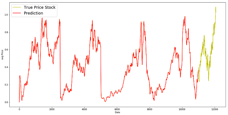
EMA is a great model for this dataset. Ideally the pattern of the True data should have been followed in the prediction model.
We coded from range to 1 to N-1 and put all the averaged values in the running mean. We used dense as 0.5 and then multiply it with the running average.
LSTM
class Generator(object):

    def __init__(self,prices,batch_size,num_unroll): #helps to generate data
        self._prices = prices
        self._prices_length = len(self._prices) - num_unroll
        self._batch_size = batch_size
        self._num_unroll = num_unroll
        self._segments = self._prices_length //self._batch_size
        self._cursor = [offset * self._segments for offset in range(self._batch_size)]

    def next(self):   #which will output a set of num_unrollings batches of input data obtained sequentially, where a batch of data is of size [batch_size, 1].

        batch_data = np.zeros((self._batch_size),dtype=np.float32)  #Then each batch of input data will have a corresponding output batch of data.
        batch_labels = np.zeros((self._batch_size),dtype=np.float32)

        for b in range(self._batch_size):   #create batches
            if self._cursor[b]+1>=self._prices_length:
                self._cursor[b] = np.random.randint(0,(b+1)*self._segments)

            batch_data[b] = self._prices[self._cursor[b]]
            batch_labels[b]= self._prices[self._cursor[b]+np.random.randint(1,5)]

            self._cursor[b] = (self._cursor[b]+1)%self._prices_length

        return batch_data,batch_labels

    def unroll(self):   #roll out the batches generated in form of data and labels

        unroll_data,unroll_labels = [],[]
        init_data, init_label = None,None
        for ui in range(self._num_unroll):

            data, labels = self.next()

            unroll_data.append(data)
            unroll_labels.append(labels)

        return unroll_data, unroll_labels

    def reset_indices(self): #get prices length
        for b in range(self._batch_size):
            self._cursor[b] = np.random.randint(0,min((b+1)*self._segments,self._prices_length-1))


dg = Generator(train,5,5)
u_data, u_labels = dg.unroll()

for ui,(dat,lbl) in enumerate(zip(u_data,u_labels)):
    print('\n\nUnrolled index %d'%ui)
    dat_ind = dat
    lbl_ind = lbl
    print('\tInputs: ',dat )
    print('\n\tOutput:',lbl)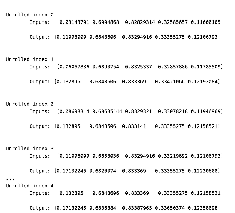
The beginning of the code forms a group called Generator which is used to produce information for a set of prices. The __init__ function establishes the initial preferences, such as the prices, amount of data in each batch, and number of consecutive groups batches of information. The following function is used to display a set of num_unrollings batches of input information that are obtained in order, where each batch has a size of [batch_size, 1].
This is done by making an array of zeroes with the size of batch_size and filling it with values from the prices group. In the same way, the function also produces an array of zeroes for the corresponding output batch of information. The for loop in the next function forms batches of information by randomly choosing a section from the prices group and completing the batch_data with the values from that section. The batch_labels array is also filled with the corresponding values from the prices group, one step ahead. This pattern is repeated for each batch by updating the cursor variable.
The unroll function performs the batches that are produced in the form of information and labels. It creates two empty lists to save the unrolled info and labels. The for loop goes through the num_unrollings and calls the following function to obtain the batch info and label. Then, these are added to the unroll info and label lists and given back in the end. The reset_indices function is used to return the cursor indices to a random position within the prices array. This ensures that the batches are randomly chosen each time the code is run. Lastly, an example of the Generator group is made with the given preferences and the unroll function is used to obtain the unrolled info and labels. This data is then published for each step.
Tewaking Hyperparameters
D = 1 # Dimensionality of the data. Since our data is 1-D this would be 1
num_unrollings = 50 # Number of time steps you look into the future.
batch_size = 500 # Number of samples in a batch
num_nodes = [200,200,150] # Number of hidden nodes in each layer of the deep LSTM stack we're using
n_layers = len(num_nodes) # number of layers
dropout = 0.2 # dropout amount

tf.reset_default_graph() # This is important in case you run this multiple times
This program sets up and assigns the values for the variables num_nodes and dropout. Firstly, it creates and sets five variables: D, num_unrollings, batch_size, num_nodes, and dropout, which will be used for future calculations. After that, it resets the graph with the command tf.reset_default_graph, which is important in case the program is run multiple times. This ensures that the numbers and equations are reset before each run. Next, it establishes the array for num_nodes with three numbers representing the amount of hidden nodes in each layer of the deep LSTM stack it will utilize. The following line uses the len function to calculate the total layers based on the num_nodes array. Lastly, the code assigns a value to the dropout variable, which randomly turns off neurons during training in order to avoid overfitting. Together, this program sets up and initializes all the necessary variables for the upcoming calculations.
Spliting the train into input and output and then we define them.
train_inputs, train_outputs = [],[]

# You unroll the input over time defining placeholders for each time step
for ui in range(num_unrollings):
    train_inputs.append(tf.placeholder(tf.float32, shape=[batch_size,D],name='train_inputs_%d'%ui))
    train_outputs.append(tf.placeholder(tf.float32, shape=[batch_size,1], name = 'train_outputs_%d'%ui))
This code is creating new lists called train_inputs and train_outputs that do not contain any data at the moment. To make things more clear, a for loop is being used to go through a certain number of steps, and for each step a placeholder is made. A placeholder is like a spot where you can put data, kind of like a fill-in-the-blank. Each placeholder is given a name that is different from the others, and is based on the number of the step that its being made for. This process is then repeated for train_outputs, but the placeholder that is made here is shaped differently. At the end of the for loop, the two lists now have placeholders for all the data that will be used during training. These placeholders will be filled with actual data during the training process.
Declare a single lstm cell use tensorflow
lstm_cells = [
    tf.contrib.rnn.LSTMCell(num_units=num_nodes[li],
                            state_is_tuple=True,
                            initializer= tf.contrib.layers.xavier_initializer()
                           )
 for li in range(n_layers)]

drop_lstm_cells = [tf.contrib.rnn.DropoutWrapper(
    lstm, input_keep_prob=1.0,output_keep_prob=1.0-dropout, state_keep_prob=1.0-dropout
) for lstm in lstm_cells]
drop_multi_cell = tf.contrib.rnn.MultiRNNCell(drop_lstm_cells)
multi_cell = tf.contrib.rnn.MultiRNNCell(lstm_cells)

w = tf.get_variable('w',shape=[num_nodes[-1], 1], initializer=tf.contrib.layers.xavier_initializer())
b = tf.get_variable('b',initializer=tf.random_uniform([1],-0.1,0.1))
The network uses a type of cell called LSTM Long Short-Term Memory to work. First, the program makes a list of LSTM cells. Each cell has a certain number of parts, and their starting values are set with the Xavier method. This happens for all the layers in the network. Then, a new list is made by wrapping each LSTM cell with a DropoutWrapper. This helps the network learn better by randomly dropping some parts with a certain chance. The next step is to make one big cell called a MultiRNNCell. This cell has many of the LSTM cells from before inside of it. This is done for both the list with dropout and the one without dropout. After that, the program creates two things called w and b, which stand for the parts that control the network. w starts with the Xavier method, and b is made with random numbers between -0.1 and 0.1. Later, these things will help the network learn how the input information is connected to the output information.
# Create cell state and hidden state variables to maintain the state of the LSTM
a1, b1 = [],[]
initial_state = []
for li in range(n_layers):
  a1.append(tf.Variable(tf.zeros([batch_size, num_nodes[li]]), trainable=False))
  b1.append(tf.Variable(tf.zeros([batch_size, num_nodes[li]]), trainable=False))
  initial_state.append(tf.contrib.rnn.LSTMStateTuple(a1[li], b1[li]))

# Do several tensor transofmations, because the function dynamic_rnn requires the output to be of
# a specific format.
all_inputs = tf.concat([tf.expand_dims(t,0) for t in train_inputs],axis=0)

# all_outputs is [seq_length, batch_size, num_nodes]
all_lstm_outputs, state = tf.nn.dynamic_rnn(
    drop_multi_cell, all_inputs, initial_state=tuple(initial_state),
    time_major = True, dtype=tf.float32)

all_lstm_outputs = tf.reshape(all_lstm_outputs, [batch_size*num_unrollings,num_nodes[-1]])

all_outputs = tf.nn.xw_plus_b(all_lstm_outputs,w,b)

split_outputs = tf.split(all_outputs,num_unrollings,axis=0)
This piece of code is organizing and working with necessary elements for utilizing a LSTM Long Short-Term Memory neural network. To start, two lists, a1 and b1, are made to hold the cell state and hidden state of the LSTM. These states will be updated and maintained as the network is trained. A special data structure called LSTMStateTuple is also made to store and manage the cell and hidden states. The initial state is a combination of the cell and hidden states from the lists a1 and b1. The next part is creating a tensor called all_inputs, which is a combination of the training inputs. The dynamic_rnn function requires a specific format for the input, so this tensor is crucial. The function is then called, with the type of cell being used a multi-cell LSTM, the input data, the initial state, and other details. This function carries out various tasks like training and updating the cell and hidden states, and producing a tensor with the networks outputs. This output tensor is reshaped and altered to match the desired format, and then separated into different tensors based on the number of training steps. This will come in handy while teaching the network, as each unrolling step represents a piece of the training data. In summary, this code sets up and organizes all the essential elements and data structures needed for working with an LSTM network, and ultimately generates the output tensors for training.
# When calculating the loss you need to be careful about the exact form, because you calculate
# loss of all the unrolled steps at the same time
# Therefore, take the mean error or each batch and get the sum of that over all the unrolled steps
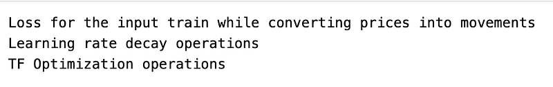
print('Loss for the input train while converting prices into movements')
loss = 0.0
with tf.control_dependencies([tf.assign(a1[li], state[li][0]) for li in range(n_layers)]+
[tf.assign(b1[li], state[li][1]) for li in range(n_layers)]):
for ui in range(num_unrollings):
loss += tf.reduce_mean(0.5*(split_outputs[ui]-train_outputs[ui])**2)
print('Learning rate decay operations')
global_step = tf.Variable(0, trainable=False)
inc_gstep = tf.assign(global_step,global_step + 1)
tf_learning_rate = tf.placeholder(shape=None,dtype=tf.float32)
tf_min_learning_rate = tf.placeholder(shape=None,dtype=tf.float32)
learning_rate = tf.maximum(
tf.train.exponential_decay(tf_learning_rate, global_step, decay_steps=1, decay_rate=0.5, staircase=True),
tf_min_learning_rate)
# Optimizer.
print('TF Optimization operations')
optimizer = tf.train.AdamOptimizer(learning_rate)
gradients, v = zip(*optimizer.compute_gradients(loss))
gradients, _ = tf.clip_by_global_norm(gradients, 5.0)
optimizer = optimizer.apply_gradients(
zip(gradients, v))
First, the program kindly informs the user about what its doing. Then, it sets the loss to 0.0. Afterwards, it uses a special function to assign values to a1 and b1 from the main state variable. This happens for each layer of the neural network. Then, it goes through a loop a certain number of times, calculating the loss at each step using a specific formula. After that, a message appears about how the learning rate is being adjusted. To keep track of the progress, a global step is created and incremented each time. A placeholder is also made for the learning rate, along with a minimum rate. Using a special formula, the code determines the learning rate using the highest value possible. This learning rate is then used in the optimization process, where an AdamOptimizer is used to calculate the gradients and limit them to a maximum value of 5.0.
Make Simple Predictions For the Above Model
 print('Defining prediction related TF functions')

sample_inputs = tf.placeholder(tf.float32, shape=[1,D])

# Maintaining LSTM state for prediction stage
sample_c, sample_h, initial_sample_state = [],[],[]
for li in range(n_layers):
  sample_c.append(tf.Variable(tf.zeros([1, num_nodes[li]]), trainable=False))
  sample_h.append(tf.Variable(tf.zeros([1, num_nodes[li]]), trainable=False))
  initial_sample_state.append(tf.contrib.rnn.LSTMStateTuple(sample_c[li],sample_h[li]))

reset_sample_states = tf.group(*[tf.assign(sample_c[li],tf.zeros([1, num_nodes[li]])) for li in range(n_layers)],
                               *[tf.assign(sample_h[li],tf.zeros([1, num_nodes[li]])) for li in range(n_layers)])

sample_outputs, sample_state = tf.nn.dynamic_rnn(multi_cell, tf.expand_dims(sample_inputs,0),
                                   initial_state=tuple(initial_sample_state),
                                   time_major = True,
                                   dtype=tf.float32)

with tf.control_dependencies([tf.assign(sample_c[li],sample_state[li][0]) for li in range(n_layers)]+
                              [tf.assign(sample_h[li],sample_state[li][1]) for li in range(n_layers)]):
  sample_prediction = tf.nn.xw_plus_b(tf.reshape(sample_outputs,[1,-1]), w, b)

print('\tAll done')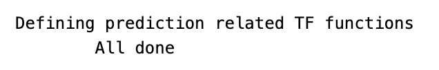
This piece of code begins by displaying a message that informs us of the TensorFlow functions involved in predicting. After that, a space is created in the TensorFlow for a one-dimensional array of numbers with decimal points shape=[1,D]. This allows for inputting data samples during the prediction process. The next part of the code deals with setting up a state for the prediction stage, called Long-Short Term Memory LSTM. This helps to keep track of important information during predictions.
A loop is used to go through the specified number of layers n_layers and for each layer, a list is created to store the sample values for the cell and hidden states sample_c and sample_h. These lists are initially filled with zeros with a size of 1 x num_nodes[li], where li stands for the layer index. Once the lists are ready, another list called initial_sample_state is created to hold the LSTMStateTuple for each layer. This is done by using the function LSTMStateTuple and passing in the current layers sample_c and sample_h values. This tuple represents the previous cell and hidden states for the current layer. Next, a set of operations is defined using the function tf.group. This set is used to reset the sample states to all zeros after making a prediction.
The first set of operations in this set uses a loop to assign all the elements in the sample_c list to zeros with dimensions of 1 x num_nodes[li], where li is the layer index. This is repeated for the sample_h list. With the sample states all reset to zeros, the next step is to run the LSTM with the sample inputs using the function dynamic_rnn from TensorFlow. This function takes in the LSTM cell multi_cell, the sample inputs, which have been expanded to have an extra dimension, and the initial state for each layer. The parameter time_major is set to True, which shows that the inputs provided are in the shape [time_steps, batch_size, input_size]. The output of this function is a tuple that contains the outputs and states for the predictions.
The final step in this code is to specify that we want to update the sample states after a prediction has been made. This is done using the function tf.control_dependencies, which states the operations that must be completed before the sample_prediction can be evaluated. These operations include assigning the sample_c and sample_h lists using the sample_state values. Lastly, the sample_prediction is defined using the operation XW plus B on the rearranged sample_outputs using the weights w and the bias b matrices. The print statement is used to let us know that the code has finished running.
Create the training model.
epochs = 50
valid_summary = 1 # Interval you make test predictions

n_predict_once = 50 # Number of steps you continously predict for

train_seq_length = train.size # Full length of the training data

train_mse_ot = [] # Accumulate Train losses
test_mse_ot = [] # Accumulate Test loss
predictions_over_time = [] # Accumulate predictions

session = tf.InteractiveSession()

tf.global_variables_initializer().run()

# Used for decaying learning rate
loss_nondecrease_count = 0
loss_nondecrease_threshold = 2 # If the test error hasn't increased in this many steps, decrease learning rate

print('Initialized')
average_loss = 0

# Define data generator
data_gen = Generator(train,batch_size,num_unrollings)

x_axis_seq = []

# Points you start our test predictions from
test_points_seq = np.arange(11000,12000,50).tolist()

for ep in range(epochs):

    #Training
    for step in range(train_seq_length//batch_size):

        u_data, u_labels = data_gen.unroll()

        feed_dict = {}
        for ui,(dat,lbl) in enumerate(zip(u_data,u_labels)):
            feed_dict[train_inputs[ui]] = dat.reshape(-1,1)
            feed_dict[train_outputs[ui]] = lbl.reshape(-1,1)

        feed_dict.update({tf_learning_rate: 0.0001, tf_min_learning_rate:0.000001})

        _, l = session.run([optimizer, loss], feed_dict=feed_dict)

        average_loss += l

    #Validation
    if (ep+1) % valid_summary == 0:

      average_loss = average_loss/(valid_summary*(train_seq_length//batch_size))

      # The average loss
      if (ep+1)%valid_summary==0:
        print('Average loss at step %d: %f' % (ep+1, average_loss))

      train_mse_ot.append(average_loss)

      average_loss = 0 # reset loss

      predictions_seq = []

      mse_test_loss_seq = []

      #Updating State and Making Predicitons
      for w_i in test_points_seq:
        mse_test_loss = 0.0
        our_predictions = []

        if (ep+1)-valid_summary==0:
          # Only calculate x_axis values in the first validation epoch
          x_axis=[]

        # Feed in the recent past behavior of stock prices
        # to make predictions from that point onwards
        for tr_i in range(w_i-num_unrollings+1,w_i-1):
          current_price = all_avg_data[tr_i]
          feed_dict[sample_inputs] = np.array(current_price).reshape(1,1)
          _ = session.run(sample_prediction,feed_dict=feed_dict)

        feed_dict = {}

        current_price = all_avg_data[w_i-1]

        feed_dict[sample_inputs] = np.array(current_price).reshape(1,1)

        # Make predictions for this many steps
        # Each prediction uses previous prediciton as it's current input
        for pred_i in range(n_predict_once):

          pred = session.run(sample_prediction,feed_dict=feed_dict)

          our_predictions.append(np.asscalar(pred))

          feed_dict[sample_inputs] = np.asarray(pred).reshape(-1,1)

          if (ep+1)-valid_summary==0:
            # Only calculate x_axis values in the first validation epoch
            x_axis.append(w_i+pred_i)

          mse_test_loss += 0.5*(pred-all_avg_data[w_i+pred_i])**2

        session.run(reset_sample_states)

        predictions_seq.append(np.array(our_predictions))

        mse_test_loss /= n_predict_once
        mse_test_loss_seq.append(mse_test_loss)

        if (ep+1)-valid_summary==0:
          x_axis_seq.append(x_axis)

      current_test_mse = np.mean(mse_test_loss_seq)

      # Learning rate decay logic
      if len(test_mse_ot)>0 and current_test_mse > min(test_mse_ot):
          loss_nondecrease_count += 1
      else:
          loss_nondecrease_count = 0

      if loss_nondecrease_count > loss_nondecrease_threshold :
            session.run(inc_gstep)
            loss_nondecrease_count = 0
            print('\tDecreasing learning rate by 0.5')

      test_mse_ot.append(current_test_mse)
      print('\tTest MSE: %.5f'%np.mean(mse_test_loss_seq))
      predictions_over_time.append(predictions_seq)
      print('\tFinished Predictions')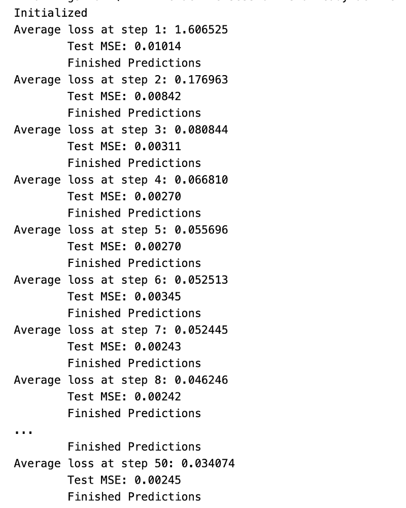
To begin, we set the number of times the model will learn epochs to 50 and decide how often we want to test its predictions valid_summary. We also determine how many steps to predict at once n_predict_once, the length of our training data train_seq_length, and create empty lists to keep track of train and test losses, as well as our predictions. Our goal is to create a successful model, so we start by opening a Tensorflow session and setting up variables for a decreasing learning rate.
Next, we use our training data to create a data generator and make two lists for the x-axis and test points. Then, we enter a loop that will run for the number of epochs we specified. In this loop, we first train the model by generating a new set of data and then use it to update our models performance. After completing this training, the code checks if its time to evaluate the model. If so, it calculates the average loss and prints it. Then, it resets the average loss and creates empty lists for our predictions and test loss. Moving on, we enter another loop to make predictions.
For each prediction, we give the model previously recorded stock price data and it predicts the stock price for the next time step. These predicted values are then stored in our predictions list and the test loss is calculated. As the loop continues, we check if its the first time were evaluating the model, and if so, we add the x-axis values. Then, we evaluate the current mean squared error MSE and compare it to the previous MSE. If the current MSE is higher, we decrease the learning rate to improve the models performance. Lastly, we print the current MSE and add the predictions from this epoch to our overall predictions list. This loop continues for the specified number of epochs and the final predictions are stored in the list predictions_over_time.
Plot Tensorflow Prediction Plot
best_prediction_epoch = 49 # replace this with the epoch that you got the best results when running the plotting code

plt.figure(figsize = (18,18))
plt.subplot(2,1,1)
plt.plot(range(df.shape[0]),all_avg_data,color='y',label='data')

# Plotting how the predictions change over time
# Plot older predictions with low alpha and newer predictions with high alpha
start_alpha = 0.25
alpha  = np.arange(start_alpha,1.1,(1.0-start_alpha)/len(predictions_over_time[::3]))
for p_i,p in enumerate(predictions_over_time[::3]):
    for xval,yval in zip(x_axis_seq,p):
        plt.plot(xval,yval,color='b',alpha=alpha[p_i],label='stock price movement change')

plt.title('Different test prediction models',fontsize=18)
plt.xlabel('Days',fontsize=18)
plt.ylabel('avg Price',fontsize=18)
plt.xlim(11000,12500)

plt.subplot(2,1,2)

# Predicting the best test prediction you got
plt.plot(range(df.shape[0]),all_avg_data,color='g',label='predictions')
for xval,yval in zip(x_axis_seq,predictions_over_time[best_prediction_epoch]):
    plt.plot(xval,yval,color='b',label='change in price movement')

plt.title('Top Predictions wrt time',fontsize=18)
plt.xlabel('Days',fontsize=18)
plt.ylabel('avg Price',fontsize=18)
plt.xlim(11000,12500)
plt.show()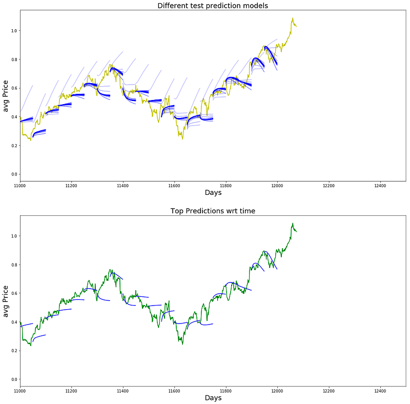
This program helps us create graphs to see how accurate our stock price predictions are over a certain time period. The first part assigns the most accurate prediction timeframe to a variable called best_prediction_epoch. Then, we create a graph with dimensions of 18x18 and add two smaller graphs to it using the subplot function. The first graph shows the data points from our dataset, while the second one shows the predictions made by our model. For the first graph, we use a line graph to show the average stock price over time. The color yellow is used for this line and it is labeled as data. Next, we use a loop to plot the predictions made by our model over time. We get the x and y values from the predictions_over_time variable, which has the predicted stock prices at different intervals.
To make it easier to see the changes in predictions over time, we adjust the transparency of the lines using the variables start_alpha and alpha. Older predictions have lower transparency, while newer ones have higher transparency. In the second graph, we follow the same steps to plot the predictions, but only for the best prediction timeframe. This is done by using the best_prediction_epoch variable to access the predictions from that specific timeframe. The lines are plotted in green and labeled as predictions. This graph allows us to closely compare the predictions from the best timeframe with the actual data. Finally, we use the subplot function to arrange the two graphs in a 2x1 grid and adjust the x and y limits to focus on a specific range of data. The final result is shown using the show function.
Make a Generator Sequence Again.
class Generator(object):

    def __init__(self,prices,batch_size,num_unroll): #helps to generate data
        self._prices = prices
        self._prices_length = len(self._prices) - num_unroll
        self._batch_size = batch_size
        self._num_unroll = num_unroll
        self._segments = self._prices_length //self._batch_size
        self._cursor = [offset * self._segments for offset in range(self._batch_size)]

    def next(self):   #which will output a set of num_unrollings batches of input data obtained sequentially, where a batch of data is of size [batch_size, 1].

        batch_data = np.zeros((self._batch_size),dtype=np.float32)  #Then each batch of input data will have a corresponding output batch of data.
        batch_labels = np.zeros((self._batch_size),dtype=np.float32)

        for b in range(self._batch_size):   #create batches
            if self._cursor[b]+1>=self._prices_length:
                self._cursor[b] = np.random.randint(0,(b+1)*self._segments)

            batch_data[b] = self._prices[self._cursor[b]]
            batch_labels[b]= self._prices[self._cursor[b]+np.random.randint(1,5)]

            self._cursor[b] = (self._cursor[b]+1)%self._prices_length

        return batch_data,batch_labels

    def unroll(self):   #roll out the batches generated in form of data and labels

        unroll_data,unroll_labels = [],[]
        init_data, init_label = None,None
        for ui in range(self._num_unroll):

            data, labels = self.next()

            unroll_data.append(data)
            unroll_labels.append(labels)

        return unroll_data, unroll_labels

    def reset_indices(self): #get prices length
        for b in range(self._batch_size):
            self._cursor[b] = np.random.randint(0,min((b+1)*self._segments,self._prices_length-1))


dg = Generator(train,5,5)
u_data, u_labels = dg.unroll()

for ui,(dat,lbl) in enumerate(zip(u_data,u_labels)):
    print('\n\nUnrolled index %d'%ui)
    dat_ind = dat
    lbl_ind = lbl
    print('\tInputs: ',dat )
    print('\n\tOutput:',lbl)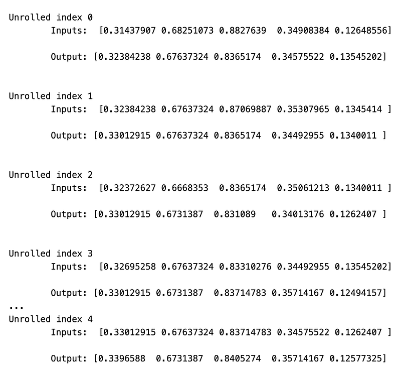
This piece of code is designed to produce data for a neural network. It contains a class called Generator that has three properties: prices, batch size, and num_unroll. The prices property stores a list of prices, the batch size determines the input data size for each batch, and the num_unroll decides the number of batches generated in sequence. The __init__ function is used to set up the Generator class by taking in the prices, batch size, and num_unroll and assigning them to their respective properties. It also calculates the number of segments based on the prices, batch size, and num_unroll.
The cursor property keeps track of the current position in the prices list. The next function generates a batch of input data and its corresponding output data. It starts by creating two arrays of zeros: one for the batch data, and the other for the labels. Then, it goes through the batch size and randomly selects data points from the prices list to create the batches. If the cursor reaches the end of the prices list, it goes back to a random position within the range of the batch.
The batch labels are chosen by randomly selecting a data point from 1 to 5 within the next data points in the prices list. This process continues until the batch size is reached. After that, the batch data and labels are returned. The unroll function creates the batches of data and labels in a continuous format by calling the next function and adding them to two arrays: unroll_data and unroll_labels. These arrays hold all the batches generated in sequence. Finally, the reset_indices function resets the cursor to a random position within the prices list. This is done before generating each batch to prevent any bias towards the end of the prices list.
Run Another Model Changing Hyperparameter And Epoch
D = 1 # Dimensionality of the data. Since our data is 1-D this would be 1
num_unrollings = 75
batch_size = 300
num_nodes = [250,250,175] # Number of hidden nodes in each layer of the deep LSTM stack we're using
n_layers = len(num_nodes) # number of layers
dropout = 0.2 # dropout amount

tf.reset_default_graph() # This is important in case you run this multiple times
This piece of code creates a special type of computer program called a neural network, using a deep technology called LSTM. Its set up to work with data that has one dimension, meaning its only measured in one direction. The data will be organized in groups of 300, with 75 steps in each group. The LSTM has different layers, and in each one there are 250, 250, and 175 hidden parts respectively. The number of layers is determined by looking at the num_nodes list, which in this case has 3 elements. We also make sure not to overwork the program by having a safety measure of 0.2. Lastly, the tf.reset_default_graph function gets things ready for us to start building our program all over again if needed.
lstm_cells = [
    tf.contrib.rnn.LSTMCell(num_units=num_nodes[li],
                            state_is_tuple=True,
                            initializer= tf.contrib.layers.xavier_initializer()
                           )
 for li in range(n_layers)]

drop_lstm_cells = [tf.contrib.rnn.DropoutWrapper(
    lstm, input_keep_prob=1.0,output_keep_prob=1.0-dropout, state_keep_prob=1.0-dropout
) for lstm in lstm_cells]
drop_multi_cell = tf.contrib.rnn.MultiRNNCell(drop_lstm_cells)
multi_cell = tf.contrib.rnn.MultiRNNCell(lstm_cells)

w = tf.get_variable('w',shape=[num_nodes[-1], 1], initializer=tf.contrib.layers.xavier_initializer())
b = tf.get_variable('b',initializer=tf.random_uniform([1],-0.1,0.1))
This piece of code is used to set up and start using LSTM cells in a recurrent neural network. It first makes a list called lstm_cells by looping through the number of layers in the network. Then, it creates each LSTM cell within the loop using tf.contrib.rnn.LSTMCell. The cells number of hidden units is set and the state is made into a tuple. Additionally, it uses tf.contrib.layers.xavier_initializer to set the cells weights. Another list, drop_lstm_cells, is then made through another loop. This loop goes through the previously created LSTM cells and uses tf.contrib.rnn.DropoutWrapper to add a dropout layer to each cell. This layer minimizes overfitting by randomly omitting certain inputs and outputs during training. When all the cells are finished, a tf.contrib.rnn.MultiRNNCell combines the drop_lstm_cells list, creating one multi-layer LSTM cell.
This final cell is used in the network. A separate multi-layer LSTM cell is also made without the dropout layer using the lstm_cells list. Next, two variables, w and b, are made with tf.get_variable. w is used to hold the weights for the output layer and is initialized by using tf.contrib.layers.xavier_initializer. b is used to store the bias and is also initialized with random values ranging from -0.1 to 0.1 using tf.random_uniform.
# Create cell state and hidden state variables to maintain the state of the LSTM
a1, b1 = [],[]
initial_state = []
for li in range(n_layers):
  a1.append(tf.Variable(tf.zeros([batch_size, num_nodes[li]]), trainable=False))
  b1.append(tf.Variable(tf.zeros([batch_size, num_nodes[li]]), trainable=False))
  initial_state.append(tf.contrib.rnn.LSTMStateTuple(a1[li], b1[li]))

# Do several tensor transofmations, because the function dynamic_rnn requires the output to be of
# a specific format.
all_inputs = tf.concat([tf.expand_dims(t,0) for t in train_inputs],axis=0)

# all_outputs is [seq_length, batch_size, num_nodes]
all_lstm_outputs, state = tf.nn.dynamic_rnn(
    drop_multi_cell, all_inputs, initial_state=tuple(initial_state),
    time_major = True, dtype=tf.float32)

all_lstm_outputs = tf.reshape(all_lstm_outputs, [batch_size*num_unrollings,num_nodes[-1]])

all_outputs = tf.nn.xw_plus_b(all_lstm_outputs,w,b)

split_outputs = tf.split(all_outputs,num_unrollings,axis=0)
This piece of code helps us keep track of the status of cells and hidden layers in a special type of neural network called LSTM. We use two variables, a1 and b1, to represent the cell state and hidden state in each layer of the LSTM. These variables are set to zero and cannot be changed during training. The code then rearranges the input data so that it can be used by the LSTM. It combines all the training inputs and adds a new dimension to account for the length of the sequence. This is important for the later step of using the dynamic_rnn function. This function takes in the LSTM, the prepared input, and the starting state, and returns a tuple containing the cell and hidden states for each layer.
The outputs of this function are also organized in a specific way by combining the sequence length and batch size into one dimension. We then use weights and a bias term to process these outputs using the xw_plus_b function. Finally, the outputs are separated into their original format, with each one representing the result for a particular time step. This whole process readies the outputs to be used for further calculations or compared to the desired targets during training.
# When calculating the loss you need to be careful about the exact form, because you calculate
# loss of all the unrolled steps at the same time
# Therefore, take the mean error or each batch and get the sum of that over all the unrolled steps
print('Loss for the input train while converting prices into movements')
loss = 0.0
with tf.control_dependencies([tf.assign(a1[li], state[li][0]) for li in range(n_layers)]+
                             [tf.assign(b1[li], state[li][1]) for li in range(n_layers)]):
  for ui in range(num_unrollings):
    loss += tf.reduce_mean(0.5*(split_outputs[ui]-train_outputs[ui])**2)

print('Learning rate decay operations')
global_step = tf.Variable(0, trainable=False)
inc_gstep = tf.assign(global_step,global_step + 1)
tf_learning_rate = tf.placeholder(shape=None,dtype=tf.float32)
tf_min_learning_rate = tf.placeholder(shape=None,dtype=tf.float32)

learning_rate = tf.maximum(
    tf.train.exponential_decay(tf_learning_rate, global_step, decay_steps=1, decay_rate=0.5, staircase=True),
    tf_min_learning_rate)

# Optimizer.
print('TF Optimization operations')
optimizer = tf.train.AdamOptimizer(learning_rate)
gradients, v = zip(*optimizer.compute_gradients(loss))
gradients, _ =  tf.clip_by_global_norm(gradients, 5.0)
optimizer = optimizer.apply_gradients(
    zip(gradients, v))
It does this by adding up all the little mistakes for each group of numbers, and then adds them all together for all the times we did this. To make sure everything is done the right way, the program first gives values to two important things called a1 and b1, which we need for the math. Then, the learning speed gets slower as we do more steps using something called exponential decay. This helps us get better answers when we try to make things better. We use something called Adam to make the computer change the numbers and patterns in our brain program. To make sure the numbers dont get too big and get all out of control, we stop them at a number called 5.0. Then we use the Adam thing to finish up. This code is really important because it helps us teach our brain program to know how things move when prices change.
Training With 100 Epochs
epochs = 100
valid_summary = 1 # Interval you make test predictions

n_predict_once = 50 # Number of steps you continously predict for

train_seq_length = train.size # Full length of the training data

train_mse_ot = [] # Accumulate Train losses
test_mse_ot = [] # Accumulate Test loss
predictions_over_time = [] # Accumulate predictions

session = tf.InteractiveSession()

tf.global_variables_initializer().run()

# Used for decaying learning rate
loss_nondecrease_count = 0
loss_nondecrease_threshold = 2 # If the test error hasn't increased in this many steps, decrease learning rate

print('Initialized')
average_loss = 0

# Define data generator
data_gen = Generator(train,batch_size,num_unrollings)

x_axis_seq = []

# Points you start our test predictions from
test_points_seq = np.arange(11000,12000,50).tolist()

for ep in range(epochs):

    #Training
    for step in range(train_seq_length//batch_size):

        u_data, u_labels = data_gen.unroll()

        feed_dict = {}
        for ui,(dat,lbl) in enumerate(zip(u_data,u_labels)):
            feed_dict[train_inputs[ui]] = dat.reshape(-1,1)
            feed_dict[train_outputs[ui]] = lbl.reshape(-1,1)

        feed_dict.update({tf_learning_rate: 0.0001, tf_min_learning_rate:0.000001})

        _, l = session.run([optimizer, loss], feed_dict=feed_dict)

        average_loss += l

    #Validation
    if (ep+1) % valid_summary == 0:

      average_loss = average_loss/(valid_summary*(train_seq_length//batch_size))

      # The average loss
      if (ep+1)%valid_summary==0:
        print('Average loss at step %d: %f' % (ep+1, average_loss))

      train_mse_ot.append(average_loss)

      average_loss = 0 # reset loss

      predictions_seq = []

      mse_test_loss_seq = []

      #Updating State and Making Predicitons
      for w_i in test_points_seq:
        mse_test_loss = 0.0
        our_predictions = []

        if (ep+1)-valid_summary==0:
          # Only calculate x_axis values in the first validation epoch
          x_axis=[]

        # Feed in the recent past behavior of stock prices
        # to make predictions from that point onwards
        for tr_i in range(w_i-num_unrollings+1,w_i-1):
          current_price = all_avg_data[tr_i]
          feed_dict[sample_inputs] = np.array(current_price).reshape(1,1)
          _ = session.run(sample_prediction,feed_dict=feed_dict)

        feed_dict = {}

        current_price = all_avg_data[w_i-1]

        feed_dict[sample_inputs] = np.array(current_price).reshape(1,1)

        # Make predictions for this many steps
        # Each prediction uses previous prediciton as it's current input
        for pred_i in range(n_predict_once):

          pred = session.run(sample_prediction,feed_dict=feed_dict)

          our_predictions.append(np.asscalar(pred))

          feed_dict[sample_inputs] = np.asarray(pred).reshape(-1,1)

          if (ep+1)-valid_summary==0:
            # Only calculate x_axis values in the first validation epoch
            x_axis.append(w_i+pred_i)

          mse_test_loss += 0.5*(pred-all_avg_data[w_i+pred_i])**2

        session.run(reset_sample_states)

        predictions_seq.append(np.array(our_predictions))

        mse_test_loss /= n_predict_once
        mse_test_loss_seq.append(mse_test_loss)

        if (ep+1)-valid_summary==0:
          x_axis_seq.append(x_axis)

      current_test_mse = np.mean(mse_test_loss_seq)

      # Learning rate decay logic
      if len(test_mse_ot)>0 and current_test_mse > min(test_mse_ot):
          loss_nondecrease_count += 1
      else:
          loss_nondecrease_count = 0

      if loss_nondecrease_count > loss_nondecrease_threshold :
            session.run(inc_gstep)
            loss_nondecrease_count = 0
            print('\tDecreasing learning rate by 0.5')

      test_mse_ot.append(current_test_mse)
      print('\tTest MSE: %.5f'%np.mean(mse_test_loss_seq))
      predictions_over_time.append(predictions_seq)
      print('\tFinished Predictions')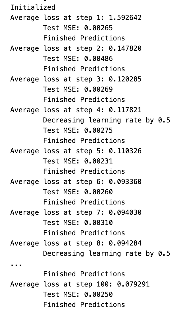
This program is created to build a neural network that learns from stock market information. The epochs, valid_summary, n_predict_once, train_seq_length, and train_mse_ot variables are used to adjust the models settings during training. To train the model, a data generator is utilized in order to create batches of data from the train information. The x_axis_seq and test_points_seq variables are responsible for selecting where the test predictions begin and end. As the model trains, the ep and step variables help to move through the data and update the weights using the backpropagation method. After each training round, there is a validation step that calculates the average loss for that round and updates the train_mse_ot variable accordingly. When its time to test the model, the code uses the current state to make predictions at specified points. The mse_test_loss variable calculates the mean squared error by comparing the predicted stock prices to the actual data. There is also a logic in place to gradually decrease the learning rate if the predicted stock prices do not show improvement over a certain number of steps. Finally, the code displays the mean squared error from the test and saves the models predictions for each round of training.
Plotting
best_prediction_epoch = 49 # replace this with the epoch that you got the best results when running the plotting code

plt.figure(figsize = (18,18))
plt.subplot(2,1,1)
plt.plot(range(df.shape[0]),all_avg_data,color='y')

# Plotting how the predictions change over time
# Plot older predictions with low alpha and newer predictions with high alpha
start_alpha = 0.25
alpha  = np.arange(start_alpha,1.1,(1.0-start_alpha)/len(predictions_over_time[::3]))
for p_i,p in enumerate(predictions_over_time[::3]):
    for xval,yval in zip(x_axis_seq,p):
        plt.plot(xval,yval,color='b',alpha=alpha[p_i])

plt.title('Different test prediction models',fontsize=18)
plt.xlabel('Date',fontsize=18)
plt.ylabel('avg Price',fontsize=18)
plt.xlim(11000,12500)

plt.subplot(2,1,2)

# Predicting the best test prediction you got
plt.plot(range(df.shape[0]),all_avg_data,color='g')
for xval,yval in zip(x_axis_seq,predictions_over_time[best_prediction_epoch]):
    plt.plot(xval,yval,color='b')

plt.title('Top Predictions wrt time',fontsize=18)
plt.xlabel('Date',fontsize=18)
plt.ylabel('avg Price',fontsize=18)
plt.xlim(11000,12500)
plt.show()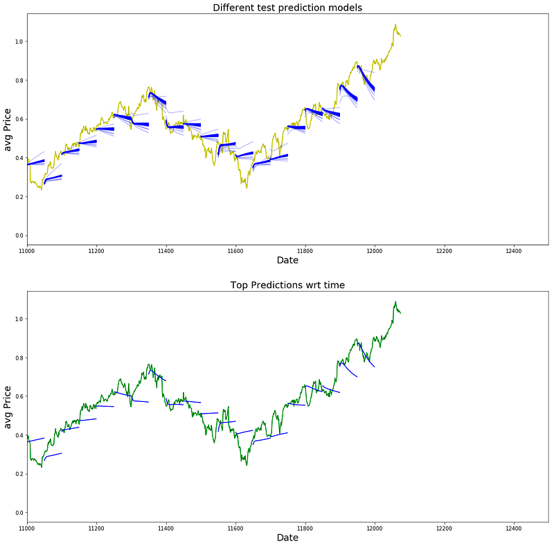
this code helps us to visualize and compare the predictions over time, specifically highlighting the best one.
That’s it folks see you In the next one.


