Low-Rank Matrix and Tensor Factorization for Speed Field Reconstruction

Introduce a sequence of matrix/tensor factorization methods and their applications to traffic flow modeling

Matrix factorization is a classical method for reconstructing missing values in matrix data. In such method, we can decompose a matrix into two factor matrices if it is possible to formulate a certain kind of optimization problem for the factorization. Tensor factorization is a higher-order extension of matrix factorization, showing a more complicated formula. In this story, we will first introduce a benchmark problem as speed field reconstruction in road traffic flow modeling. Then, on the well-defined problem, we are trying to find and provide a sequence of matrix and tensor factorization methods for imputing missing values in the given data matrix. Finally, we will provide some reconstruction results to make comparison among these matrix and tensor factorization methods.

Content:

• Motivation
• Matrix factorization

a) Optimization problem; b) Gradient descent; c) Steepest gradient descent; d) Alternating least squares; e) Comparison among GD, SGD, and ALS.

• Smoothing matrix factorization
• Tensor factorization

a) What is tensor? b) Tensor decomposition: A brief history; c) Hankel matrix & Hankel tensor; d) Hankel tensor factorization.

• Which model is better?
• Conclusion

Let’s get started!

Motivation

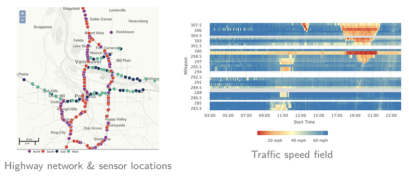
In real-world transportation systems, it is possible to gather traffic state information from highway and urban road networks. These traffic state variables include traffic volume and traffic speed. As an example, Figure 1 shows a publicly available dataset for traffic states of highways. In the right panel of Figure 1, we have a speed field in the form of matrix, showing rows as spatial locations and columns as time steps. Without loss of generality, the speed field can be represented as a matrix such as Y of size N-by-T (i.e., N rows and T columns). As can be seen, this speed field also demonstrates very strong spatial dependencies and temporal dependencies.

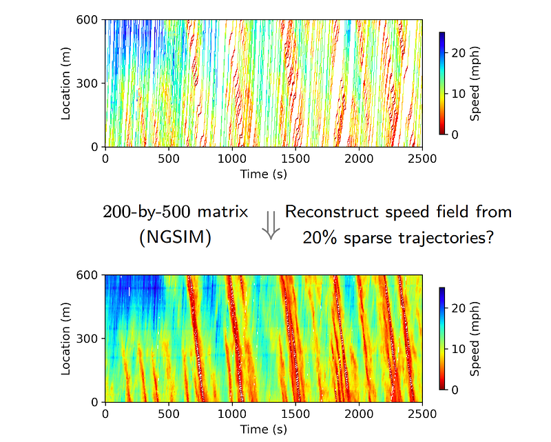
Here, we begin with a toy example to pose a well-defined speed field reconstruction problem and make it available for the following evaluation. In Figure 2, we have a sparse speed field (i.e., sparse matrix with a certain number of missing values). The modeling goal is producing a complete speed field (i.e., matrix with full entries) through a certain technique. Therefore, we have two scientific questions:

• How to learn from sparse spatiotemporal data?
• How to characterize spatial/temporal local dependencies?

Matrix Factorization

In the two decades, matrix factorization demonstrated broad applications to recommender systems, representing a class of collaborative filtering algorithms. Matrix factorization algorithms work by decomposing a given user-item rate matrix into the multiplication of user factor matrix and item factor matrix.

Optimization Problem

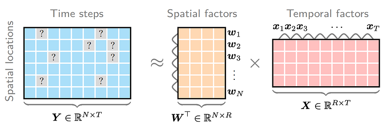
In our speed field reconstruction problem, matrix factorization also plays a very important role. Speed field data with both spatial and temporal dimensions can be reconstructed by using matrix factorization. Figure 3 shows how does matrix factorization work on the spatiotemporal speed field. If there are many missing values (i.e., the entries “?” represent missing values), it is still possible to factorize Y into the multiplication of spatial factor matrix W and temporal factor matrix X.

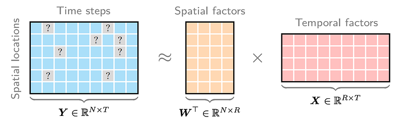
The basic idea of matrix factorization is learning factor matrices W and X from the partially observed data matrix Y. To implement such idea, we can try to write down the optimization problem of matrix factorization from a machine learning perspective:

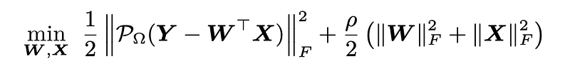
In the objective function, we have two components corresponding to both matrix factorization and regularization terms, respectively. The matrix factorization formula takes the notion of orthogonal projection, while the regularization terms take the sum of squared entries of W and X (mainly used to avoid overfitting). ρ is the weight parameter for regularization.

For notational convenience, we let the objective function be f(W, X) or f in the following description. In particular, we introduce the orthogonal projection as an important concept. The orthogonal projection is rather simple to understand if we follow this example:

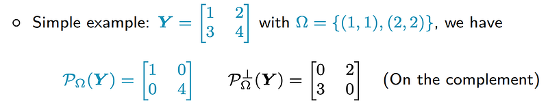
Here, if Ω = {(1, 1), (2, 2)}, then the diagonal entries of the resulted matrix would be 1 and 4, respectively.

Gradient Descent

Going back to the optimization problem of matrix factorization, we can write down the partial derivatives of the objective function f as follows,

corresponding to the spatial factor matrix W and temporal factor matrix X, respectively.

As we know, these partial derivatives can be usually regarded as gradients in machine learning. Therefore, the first impulse would be trying gradient descent (GD) to solve the optimization problem. The update rules at each iteration in the gradient descent are

where α is the step size. Updating both two equations iteratively can help us find the solution to the matrix factorization. However, one shortcoming of gradient descent is that it is not efficient in terms of convergence.

Steepest Gradient Descent

One alternative of gradient descent is the steepest gradient descent (SGD), which shows fast convergence. On the basis of the update rules in gradient descent, we need to take the following update roles at each iteration in the steepest gradient descent:

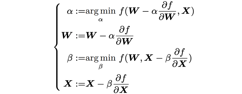
where we have two step sizes, i.e., α and β. Both two step sizes would be optimal at each iteration. It should be not hard to write down the closed-form solutions to the step sizes α and β.

Alternating Least Squares

Recall that we have partial derivatives of the objective function with respect to W and X, letting both two partial derivatives be zeros could lead to an alternating minimization scheme.

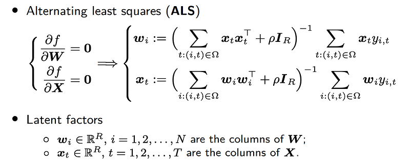
These least squares solutions allow one to develop an alternating least squares (ALS, a special case of alternating minimization) scheme for matrix factorization.

Comparison Among GD, SGD, and ALS

Putting gradient descent (GD), steepest gradient descent (SGD), and alternating least squares (ALS) together, we can conduct fair comparison on the speed field reconstruction problem for numerically checking the objective function f in the iterative process of all three optimization schemes.

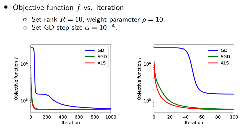
We set some preliminary parameters (including rank R and weight parameter ρ). As can be seen, we have the following findings:

• In the first 1,000 iterations, SGD and ALS are better than GD in terms of convergence.
• In the first 100 iterations, ALS is better than SGD in terms of convergence.

Figure 4 shows some intuitive results achieved by matrix factorization models. These matrix factorization can be used to reconstruct the sparse speed field and produce a complete one.

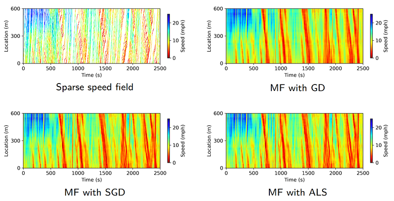
Since the speed field is a toy example, it is hard to identify which optimization scheme of matrix factorization is better. In what follows, we give some reconstruction results on a middle-size dataset.

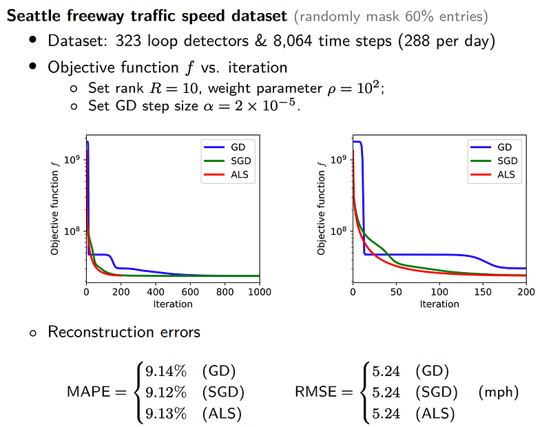
Of these results, it seems that MF with different optimization schemes have very similar performance. But in terms of convergence, ALS is the best among all three schemes.

Smoothing Matrix Factorization (SMF)

As mentioned above, matrix factorization allows one to reconstruct a sparse speed field. But actually, the performance of matrix factorization can be improved due to the strong spatial/temporal local dependencies. By doing so, we provide a new framework of matrix factorization in Figure 5.

The specific modeling target is incorporating side information by smoothing (or say first-order differencing on both W and X). The formula of first-order differencing would be

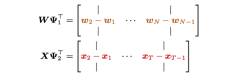
In this case, it is necessary to define a certain kind of matrix as this one:

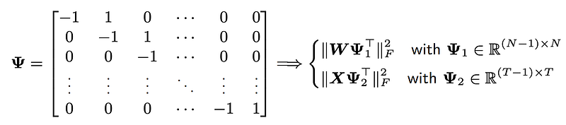
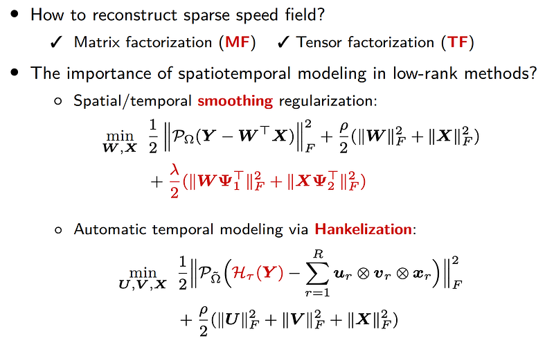
Now, it is time to take into account smoothing regularization terms for building our smoothing matrix factorization:

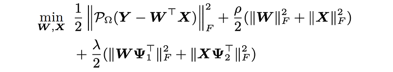
where λ is the weight parameter.

We can utilize the alternating minimization to update to the solutions to W and X iteratively. At each iteration, since the system of linear equations of W (or X) is in the form of generalized Sylvester equation, we can solve each subproblem by using the conjugate gradient method.

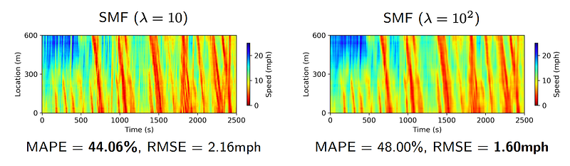
Figure 6 presents some reconstruction results produced by the smoothing matrix factorization.

Tensor Factorization

As mentioned above, we introduced both matrix factorization and smoothing matrix factorization. Both two methods allow one to produce speed field from sparse data. In what follows, we intend to provide a tensor factorization method for the speed field reconstruction problem.

What is Tensor?

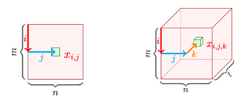
In linear algebra, a matrix consists of rows and columns, whose entries are usually indexed by both i and j as shown in Figure 7. Tensor is very different from matrix, which shows multiple dimensions. In the right panel of Figure 7, this is a third-order tensor of size m-by-n-by-t. We should use i, j, and k to represent each entry of the tensor.

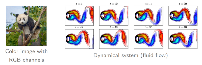
In real-world applications, we have different kinds of tensors (see Figure 8 for instance). In the left panel of Figure 8, we have a color image with a giant panda. Since each pixel has RGB (red, green, blue) channels, this color image is a third-order tensor. The right panel of Figure 8 shows a classical example of dynamical systems, here are some fluid flow snapshots in the form of matrix collected at different time slots. Putting these snapshots together along an additional dimension, we will construct a third-order tensor.

Tensor Decomposition: A Brief History

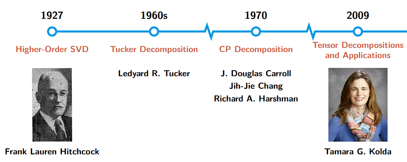
Tensor decomposition is a very classical method in matrix computations, signal processing, and machine learning, showing broad applications to real-world problems. Tensor decomposition has a rather long history, but it becomes appealing just in the past two decades. In the early stage, singular value decomposition (SVD) of matrix was introduced to tensors, namely, higher-order SVD. Today, we have two most classical formulas of tensor decomposition, i.e., Tucker decomposition (1960s) and CP decomposition (1970). There is a classical literature review paper about tensor decompositions and applications by Kolda in 2009.

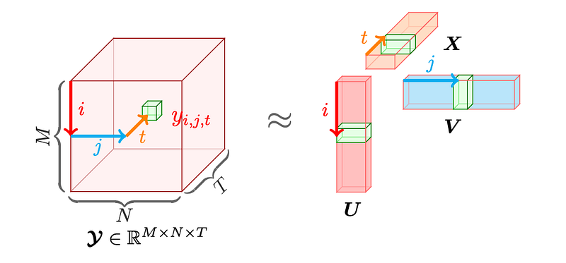
As exemplified by CP decomposition, for any given third-order tensor, we can factorize the tensor Y into the combination of three factor matrices, i.e., U, V, and X. Each factor matrix corresponds to a certain dimension of the tensor data.

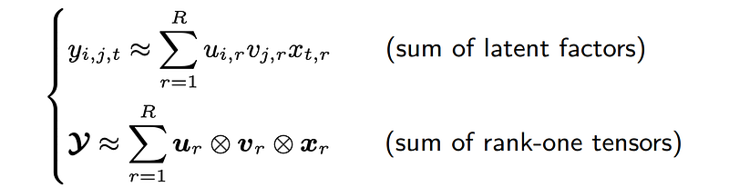
It is possible to understand CP factorization from two perspectives. On the one hand, each entry of the reconstructed tensor is the sum of latent factors. On the other hand, the reconstructed tensor is the sum of rank-one tensors. Notably, both two perspectives are also applicable to matrix factorization.

Hankel Matrix & Hankel Tensor

Since the speed field is a matrix, if we want to use tensor factorization to reconstruct sparse speed field. It is necessary to introduce an additional dimension. In what follows, we consider the Hankel structure, including Hankel matrix and Hankel tensor.

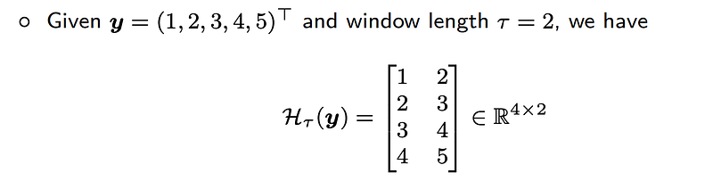
Here is a simple example on the vector y with entries 1, 2, 3, 4, and 5. If the window length of Hankel matrix (i.e., the column number) is set as 2, then the first column of the Hankel matrix would be 1, 2, 3, and 4, while the second column has entries 2, 3, 4, and 5.

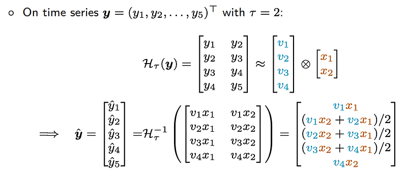
In this case, Hankel tensor is also well-suited to the time series modeling. If one assumes that the Hankel matrix can be factorized into a rank-one matrix, namely, the outer product of the vector v (four entries as v1, v2, v3, and v4) and the vector x (two entries as x1 and x2), then the estimates of the vector y captures the temporal correlations. For example, the estimate of y2 is associated with both v1 (i.e., the first entry of v) and v2 (i.e., the second entry of v).

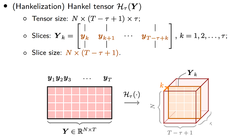
On the basis of the definition of Hankel matrix, we are proposing a certain kind of Hankel tensor defined on the matrix of size N-by-T. This Hankel tensor is of size N-by-(T-τ+1)-by-τ, each slice is a matrix consisting of vectors yk, …

Hankel Tensor Factorization (HTF)

In this case, introducing Hankel tensor on the speed field matrix allows one to capture the temporal correlations of speed field data. We can also build a Hankel tensor factorization model whose optimization problem is given by

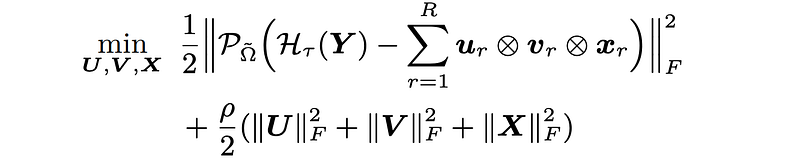
Notably, Hankel tensor factorization can achieve automatic temporal modeling.

Which Model Is Better?

We evaluate the Hankel tensor factorization on the speed field reconstruction problem and put the results of both MF and SMF in Figure 10. All three matrix/tensor factorization methods learn from the sparse speed field. We have ground truth speed field for the verification.

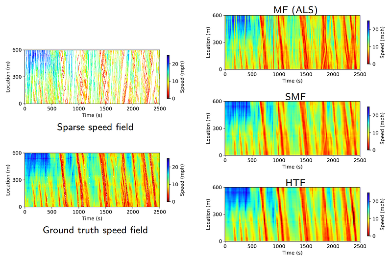
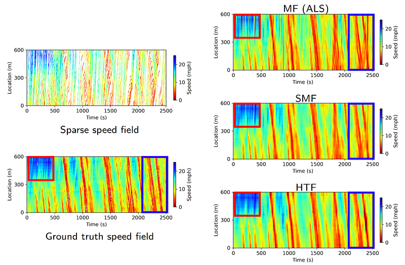
Figure 11 highlights some areas of the speed fields. It seems that the speed field achieved by HTF is more consistent with the ground truth speed field.

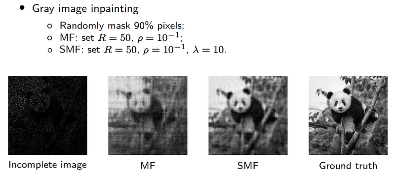
Another intuitive example is about gray image inpainting, we can test both MF and SMF for this task and find a better reconstruction from SMF.

Conclusion

In this story, we are trying to introduce some matrix and tensor factorization methods for a classical spatiotemporal reconstruction problem. Here, despite the successful performance of low-rank modeling on the speed field reconstruction problem, we highlight the importance of spatiotemporal modeling. Two kinds of spatiotemporal modeling mechanisms are available in this story, i.e., spatial/temporal smoothing regularization and automatic temporal modeling via Hankelization.

[Source #1] The content of this story is summarized from our recent slides for introducing some basic matrix/tensor factorization models to road traffic flow modeling. The slides are available at https://xinychen.github.io/slides/MF_TF_SFR.pdf

[Source #2] If you are interested in reproducing the experiments in these slides, a Jupyter Notebook with NumPy implementation is also publicly available at https://github.com/xinychen/transdim/blob/master/toy-examples/MF_TF_SFR.ipynb

If you have any feedback, feel free to let us know!