
Essential Math for Machine Learning: Low-Rank Approximation with SVD
This article is part of the series Essential Math for Machine Learning.
SVD
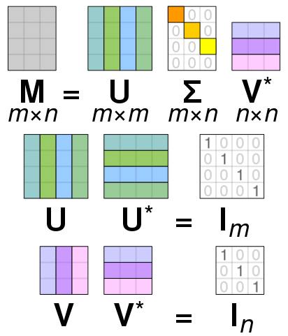
In the realm of linear algebra, the Singular Value Decomposition (SVD) stands as a fundamental tool that unveils the underlying structure within matrices. It decomposes a matrix into three distinct components, each offering unique insights:
- U: An orthogonal matrix representing the left singular vectors, capturing patterns in the rows of the original matrix.
- Σ: A diagonal matrix containing the singular values, arranged in descending order. These values quantify the importance of each corresponding singular vector.
- V*: The transpose of an orthogonal matrix representing the right singular vectors, capturing patterns in the columns.
Mathematically, SVD expresses a matrix M as:
M = UΣV*Low-Rank Approximation
Low-rank approximation is a technique that harnesses SVD to create a simplified version of a matrix while preserving its essential information. It’s achieved by retaining only the most significant singular values and their corresponding vectors.
Here’s why it’s so valuable:
- Noise Reduction: Filtering out less important information can diminish noise and highlight core patterns.
- Dimensionality Reduction: Compressing data into a lower-dimensional representation reduces computational costs and storage requirements.
- Feature Extraction: Identifying the most prominent features within a dataset can enhance analysis and modeling.
NumPy Example
NumPy, Python’s numerical powerhouse, provides seamless SVD implementation. The code is available in this Colab notebook.
import numpy as np

def create_matrix(m, n):
  '''Creates a random matrix of shape mxn for testing.'''
  M = np.random.rand(m, n)  # Generate random matrix of size m x n
  print('The original matrix M:\n', M)
  print('M shape:', M.shape)  # Print the shape for reference
  return M

def decompose_matrix(M):
  '''Decomposes the matrix M using Singular Value Decomposition (SVD).'''
  U, S, V = np.linalg.svd(M)  # Perform SVD
  print('U shape:', U.shape)
  print('S shape:', S.shape)
  print('V shape:', V.shape)

  # Adjust matrix shapes to ensure U (m x n), S (n x n), V (n x n):
  U = U[:, :S.shape[0]]  # Limit U to the number of singular values
  S = np.diag(S)  # Convert S (a vector) into a diagonal matrix
  print('Adjusted U shape:', U.shape)
  print('Adjusted S shape:', S.shape)
  print('Adjusted V shape:', V.shape)

  return U, S, V

def reconstruct_matrix(U, S, V, r):
  '''Reconstructs the matrix using the SVD components with rank r.'''
  print('\nReconstructing matrix with rank=', r)
  R = U[:, :r] @ S[:r, :r] @ V[:r, :]  # Use rank-reduced components for approximation
  print(R)
  print('R shape:', R.shape)  # Output shape of the approximated matrix
  return R

def compare_matrices(M, R):
  '''Calculates the difference and relative difference between the original and
      reconstructed matrix.'''
  D = M - R  # Element-wise difference
  M_norm = np.linalg.norm(M, 'fro')  # Frobenius norm of original matrix
  D_norm = np.linalg.norm(D, 'fro')  # Frobenius norm of difference matrix
  print('Diff:\n', np.array_str(D, precision=2, suppress_small=True))  # Print differences
  return D_norm / M_norm  # Calculate the relative difference ratio

# Test the functions with sample values:
m = 10
n = 5
M = create_matrix(m, n)  # Create the matrix

U, S, V = decompose_matrix(M)  # Decompose with SVD

R1 = reconstruct_matrix(U, S, V, n)  # Full reconstruction (using all singular values)
diff_ratio1 = compare_matrices(M, R1)
print(f'Diff ratio 1: {diff_ratio1:.2f}')

R2 = reconstruct_matrix(U, S, V, n - 1)  # Reduced-rank reconstruction
diff_ratio2 = compare_matrices(M, R2)
print(f'Diff ratio 2: {diff_ratio2:.2f}')
Explanation of Key Points:
- Rank of a matrix: The number of linearly independent rows or columns. Reducing the rank during reconstruction leads to creating a low-rank approximation of the original matrix.
- Frobenius norm: A way to calculate the “magnitude” of a matrix, treating the matrix as a long vector. It is used here to measure how different the reconstructed matrix is from the original one.
Output:
The original matrix M:
 [[0.31135826 0.42274964 0.37369816 0.27318393 0.3395049 ]
 [0.09573013 0.41568315 0.98607672 0.18737016 0.12099308]
 [0.82725089 0.78642023 0.50616054 0.02557229 0.69397554]
 [0.92327493 0.9312128  0.09507911 0.10979784 0.54611549]
 [0.73422037 0.66289384 0.13675995 0.41820362 0.45485017]
 [0.95800196 0.72963655 0.61210155 0.24766389 0.75359343]
 [0.74954623 0.24386793 0.77440318 0.96037917 0.21616432]
 [0.10595959 0.02953947 0.84582789 0.42635078 0.28987665]
 [0.63583439 0.56250889 0.73797078 0.38151526 0.97479939]
 [0.97645554 0.05086654 0.90573323 0.05414428 0.1257033 ]]
M shape: {(10, 5)}
U shape: (10, 10)
S shape: (5,)
V shape: (5, 5)
Adjusted U shape: (10, 5)
Adjusted S shape: (5, 5)
Adjusted V shape: (5, 5)

Reconstructing matrix with rank= 5
[[0.31135826 0.42274964 0.37369816 0.27318393 0.3395049 ]
 [0.09573013 0.41568315 0.98607672 0.18737016 0.12099308]
 [0.82725089 0.78642023 0.50616054 0.02557229 0.69397554]
 [0.92327493 0.9312128  0.09507911 0.10979784 0.54611549]
 [0.73422037 0.66289384 0.13675995 0.41820362 0.45485017]
 [0.95800196 0.72963655 0.61210155 0.24766389 0.75359343]
 [0.74954623 0.24386793 0.77440318 0.96037917 0.21616432]
 [0.10595959 0.02953947 0.84582789 0.42635078 0.28987665]
 [0.63583439 0.56250889 0.73797078 0.38151526 0.97479939]
 [0.97645554 0.05086654 0.90573323 0.05414428 0.1257033 ]]
R shape: (10, 5)
Diff:
 [[-0. -0. -0. -0. -0.]
 [ 0.  0. -0. -0.  0.]
 [ 0.  0.  0.  0.  0.]
 [ 0. -0.  0.  0. -0.]
 [-0.  0.  0.  0.  0.]
 [ 0.  0. -0.  0. -0.]
 [-0.  0. -0.  0.  0.]
 [ 0.  0.  0.  0.  0.]
 [ 0.  0.  0.  0.  0.]
 [-0.  0. -0.  0.  0.]]
Diff ratio 1: 0.00

Reconstructing matrix with rank= 4
[[0.32011499 0.37668989 0.3653731  0.27113115 0.38645801]
 [0.13724317 0.19732788 0.94661011 0.17763856 0.34358351]
 [0.8285426  0.77962592 0.50493251 0.02526949 0.70090163]
 [0.94319277 0.82644657 0.07614314 0.10512865 0.65291374]
 [0.74350028 0.61408225 0.12793751 0.41602819 0.50460849]
 [0.9490786  0.77657269 0.62058502 0.24975573 0.70574693]
 [0.75529316 0.21363955 0.76893956 0.95903196 0.246979  ]
 [0.09566755 0.08367476 0.85561257 0.42876347 0.23469138]
 [0.59964019 0.75288749 0.77238075 0.39       0.78072826]
 [0.96773383 0.09674206 0.91402499 0.05618885 0.07893799]]
R shape: (10, 5)
Diff:
 [[-0.01  0.05  0.01  0.   -0.05]
 [-0.04  0.22  0.04  0.01 -0.22]
 [-0.    0.01  0.    0.   -0.01]
 [-0.02  0.1   0.02  0.   -0.11]
 [-0.01  0.05  0.01  0.   -0.05]
 [ 0.01 -0.05 -0.01 -0.    0.05]
 [-0.01  0.03  0.01  0.   -0.03]
 [ 0.01 -0.05 -0.01 -0.    0.06]
 [ 0.04 -0.19 -0.03 -0.01  0.19]
 [ 0.01 -0.05 -0.01 -0.    0.05]]
Diff ratio 2: 0.12
Conclusion
SVD and low-rank approximations offer a potent toolkit for extracting meaningful information from matrices, empowering data exploration and analysis across diverse fields. Unlock their potential with NumPy and dive into a world of insights!
References
ML Algorithm: Singular Value Decomposition
https://dustinstansbury.github.io/theclevermachine/svd-data-compression


