
Logistic Regression From Scratch in Python
Machine Learning From Scratch: Part 5
In this article, we are going to implement the most commonly used Classification algorithm called the Logistic Regression. First, we will understand the Sigmoid function, Hypothesis function, Decision Boundary, the Log Loss function and code them alongside.
After that, we will apply the Gradient Descent Algorithm to find the parameters, weights and bias . Finally, we will measure accuracy and plot the decision boundary for a linearly separable dataset and a non-linearly separable dataset.
We will implement it all using Python NumPy and Matplotlib.
Notations —
n→number of featuresm→number of training examplesX→input data matrix of shape (mxn)y→true/ target value (can be 0 or 1 only)x(i), y(i)→ith training examplew→ weights (parameters) of shape (nx 1)b→bias (parameter), a real number that can be broadcasted.y_hat(y with a cap/hat)→ hypothesis (outputs values between 0 and 1)
We are going to do binary classification, so the value of y (true/target) is going to be either 0 or 1.
For example, suppose we have a breast cancer dataset with X being the tumor size and y being whether the lump is malignant(cancerous) or benign(non-cancerous). Whenever a patient visits, your job is to tell him/her whether the lump is malignant(0) or benign(1) given the size of the tumor. There are only two classes in this case.
So, y is going to be either 0 or 1.
Logistic Regression
Let’s use the following randomly generated data as a motivating example to understand Logistic Regression.
from sklearn.datasets import make_classificationX, y = make_classification(n_features=2, n_redundant=0,
n_informative=2, random_state=1,
n_clusters_per_class=1)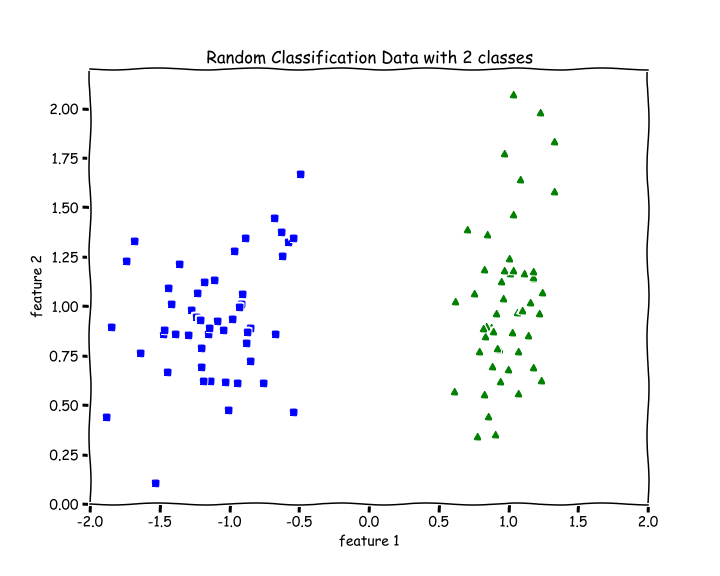
There are 2 features, n=2. There are 2 classes, blue and green.
For a binary classification problem, we naturally want our hypothesis (y_hat) function to output values between 0 and 1 which means all Real numbers from 0 to 1.
So, we want to choose a function that squishes all its inputs between 0 and 1. One such function is the Sigmoid or Logistic function.
Sigmoid or Logistic function
The Sigmoid Function squishes all its inputs (values on the x-axis) between 0 and 1 as we can see on the y-axis in the graph below.
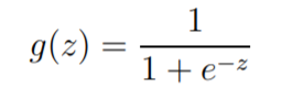
The range of inputs for this function is the set of all Real Numbers and the range of outputs is between 0 and 1.
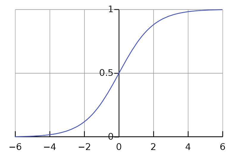
We can see that as z increases towards positive infinity the output gets closer to 1, and as z decreases towards negative infinity the output gets closer to 0.
def sigmoid(z):
    return 1.0/(1 + np.exp(-z))
Hypothesis
For Linear Regression, we had the hypothesis y_hat = w.X +b , whose output range was the set of all Real Numbers.
Now, for Logistic Regression our hypothesis is — y_hat = sigmoid(w.X + b) , whose output range is between 0 and 1 because by applying a sigmoid function, we always output a number between 0 and 1.
y_hat =
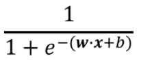
z = w.X +b
Now, you might wonder that there are lots of continuous function that outputs values between 0 and 1. Why did we choose the Logistic Function only, why not any other? Actually, there is a broader class of algorithms called Generalized Linear Models of which this is a special case. Sigmoid function falls out very naturally from it given our set of assumptions.
Loss/Cost function
For every parametric machine learning algorithm, we need a loss function, which we want to minimize (find the global minimum of) to determine the optimal parameters(w and b) which will help us make the best predictions.
For Linear Regression, we had the mean squared error as the loss function. But that was a regression problem.
For a binary classification problem, we need to be able to output the probability of y being 1(tumor is benign for example), then we can determine the probability of y being 0(tumor is malignant) or vice versa.
So, we assume that the values that our hypothesis(y_hat) outputs between 0 and 1, is a probability of y being 1, then the probability of y being 0 will be (1-y_hat) .
Remember that
yis only 0 or 1.y_hatis a number between 0 and 1.
More formally, the probability of y=1 given X , parameterized by w and b is y_hat (hypothesis). Then, logically the probability of y=0 given X , parameterized by w and b should be 1-y_hat . This can be written as —
P(y = 1 | X; w, b) = y_hat
P(y = 0 | X; w, b) = (1-y_hat)
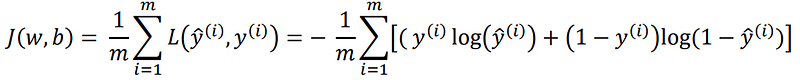
Then, based on our assumptions, we can calculate the loglikelihood of parameters using the above two equations and consequently determine the loss function which we have to minimize. The following is the Binary Coss-Entropy Loss or the Log Loss function —
For reference — Understanding the Logistic Regression and likelihood
J(w,b) is the overall cost/loss of the training set and L is the cost for ith training example.
def loss(y, y_hat):
    loss = -np.mean(y*(np.log(y_hat)) - (1-y)*np.log(1-y_hat))
    return loss
By looking at the Loss function, we can see that loss approaches 0 when we predict correctly, i.e, when y=0 and y_hat=0 or, y=1 and y_hat=1, and loss function approaches infinity if we predict incorrectly, i.e, when y=0 but y_hat=1 or, y=1 but y_hat=1.
Gradient Descent
Now that we know our hypothesis function and the loss function, all we need to do is use the Gradient Descent Algorithm to find the optimal values of our parameters like this(lr →learning rate) —
w := w-lr*dw
b := b-lr*db
where, dw is the partial derivative of the Loss function with respect to w and db is the partial derivative of the Loss function with respect to b .
dw = (1/m)*(y_hat — y).X
db = (1/m)*(y_hat — y)
Let’s write a function gradients to calculate dw and db .
See comments(#).
def gradients(X, y, y_hat):

    # X --> Input.
    # y --> true/target value.
    # y_hat --> hypothesis/predictions.
    # w --> weights (parameter).
    # b --> bias (parameter).

    # m-> number of training examples.
    m = X.shape[0]

    # Gradient of loss w.r.t weights.
    dw = (1/m)*np.dot(X.T, (y_hat - y))

    # Gradient of loss w.r.t bias.
    db = (1/m)*np.sum((y_hat - y))

    return dw, db
Decision boundary
Now, we want to know how our hypothesis(y_hat) is going to make predictions of whether y=1 or y=0. The way we defined hypothesis is the probability of y being 1 given X and parameterized by w and b .
So, we will say that it will make a prediction of —
y=1 when y_hat ≥ 0.5
y=0 when y_hat < 0.5
Looking at the graph of the sigmoid function, we see that for —
y_hat ≥ 0.5, z or w.X + b ≥ 0
y_hat < 0.5, z or w.X + b < 0
which means, we make a prediction for —
y=1 when w.X + b ≥ 0
y=0 when w.X + b < 0
So, w.X + b = 0 is going to be our Decision boundary.
The following code for plotting the Decision Boundary only works when we have only two features in
X.
def plot_decision_boundary(X, w, b):

    # X --> Inputs
    # w --> weights
    # b --> bias

    # The Line is y=mx+c
    # So, Equate mx+c = w.X + b
    # Solving we find m and c
    x1 = [min(X[:,0]), max(X[:,0])]
    m = -w[0]/w[1]
    c = -b/w[1]
    x2 = m*x1 + c

    # Plotting
    fig = plt.figure(figsize=(10,8))
    plt.plot(X[:, 0][y==0], X[:, 1][y==0], "g^")
    plt.plot(X[:, 0][y==1], X[:, 1][y==1], "bs")
    plt.xlim([-2, 2])
    plt.ylim([0, 2.2])
    plt.xlabel("feature 1")
    plt.ylabel("feature 2")
plt.title('Decision Boundary') plt.plot(x1, x2, 'y-')Normalize Function
Function to normalize the inputs. See comments(#).
def normalize(X):

    # X --> Input.

    # m-> number of training examples
    # n-> number of features
    m, n = X.shape

    # Normalizing all the n features of X.
    for i in range(n):
        X = (X - X.mean(axis=0))/X.std(axis=0)

    return X
Train Function
The train the function includes initializing the weights and bias and the training loop with mini-batch gradient descent.
See comments(#).
def train(X, y, bs, epochs, lr):

    # X --> Input.
    # y --> true/target value.
    # bs --> Batch Size.
    # epochs --> Number of iterations.
    # lr --> Learning rate.

    # m-> number of training examples
    # n-> number of features
    m, n = X.shape

    # Initializing weights and bias to zeros.
    w = np.zeros((n,1))
    b = 0

    # Reshaping y.
    y = y.reshape(m,1)

    # Normalizing the inputs.
    x = normalize(X)

    # Empty list to store losses.
    losses = []

    # Training loop.
    for epoch in range(epochs):
        for i in range((m-1)//bs + 1):

            # Defining batches. SGD.
            start_i = i*bs
            end_i = start_i + bs
            xb = X[start_i:end_i]
            yb = y[start_i:end_i]

            # Calculating hypothesis/prediction.
            y_hat = sigmoid(np.dot(xb, w) + b)

            # Getting the gradients of loss w.r.t parameters.
            dw, db = gradients(xb, yb, y_hat)

            # Updating the parameters.
            w -= lr*dw
            b -= lr*db

        # Calculating loss and appending it in the list.
        l = loss(y, sigmoid(np.dot(X, w) + b))
        losses.append(l)

    # returning weights, bias and losses(List).
    return w, b, losses
Predict Function
See comments(#).
def predict(X):

    # X --> Input.

    # Normalizing the inputs.
    x = normalize(X)

    # Calculating presictions/y_hat.
    preds = sigmoid(np.dot(X, w) + b)

    # Empty List to store predictions.
    pred_class = []
# if y_hat >= 0.5 --> round up to 1
# if y_hat < 0.5 --> round up to 1
pred_class = [1 if i > 0.5 else 0 for i in preds]
return np.array(pred_class)Training and Plotting Decision Boundary
# Training
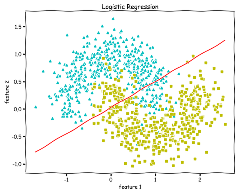
w, b, l = train(X, y, bs=100, epochs=1000, lr=0.01)# Plotting Decision Boundary
plot_decision_boundary(X, w, b)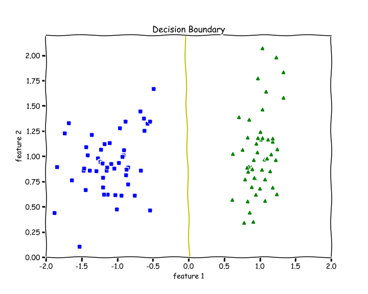
Calculating Accuracy
We check how many examples did we get right and divide it by the total number of examples.
def accuracy(y, y_hat):
    accuracy = np.sum(y == y_hat) / len(y)
return accuracyaccuracy(X, y_hat=predict(X))
>> 1.0We get an accuracy of 100%. We can see from the above decision boundary graph that we are able to separate the green and blue classes perfectly.
Testing on Non-linearly Separable Data
Let’s test out our code for data that is not linearly separable.
from sklearn.datasets import make_moonsX, y = make_moons(n_samples=100, noise=0.24)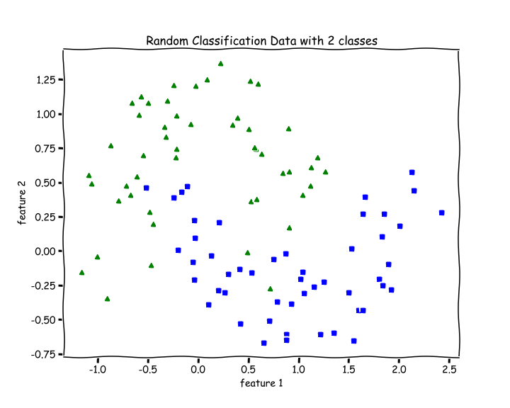
# Training
w, b, l = train(X, y, bs=100, epochs=1000, lr=0.01)
# Plotting Decision Boundary
plot_decision_boundary(X, w, b)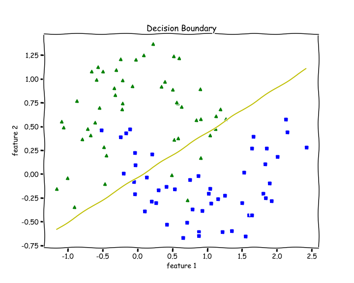
Since Logistic Regression is only a linear classifier, we were able to put a decent straight line which was able to separate as many blues and greens from each other as possible.
Let’s check accuracy for this —
accuracy(y, predict(X))
>> 0.87
87 % accuracy. Not bad.
Important Insights
When I was training the data using my code, I always got the NaN values in my losses list.
Later I discovered the I was not normalizing my inputs, and that was the reason my losses were full of NaNs.
If you are getting NaN values or overflow during training —
- Normalize your Data —
X. - Lower your Learning rate.
Thanks for reading. For questions, comments, concerns, talk to be in the response section. More ML from scratch is coming soon.
Check out the Machine Learning from scratch series —


