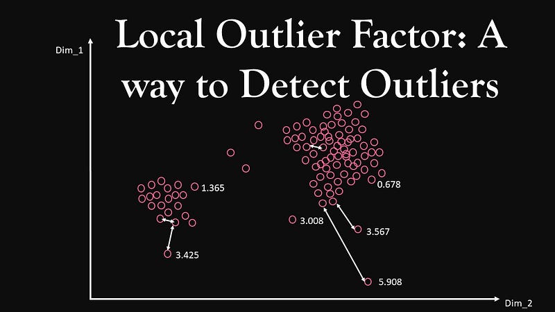
Local Outlier Factor: A way to Detect Outliers

As we Know, Outliers are patterns in the datasets that do not conform to the expected behaviour. It may appear in the dataset due to low-quality measurements, malfunctioning equipment, manual error e.t.c. The presence of outliers may create problems in building a good machine learning model.

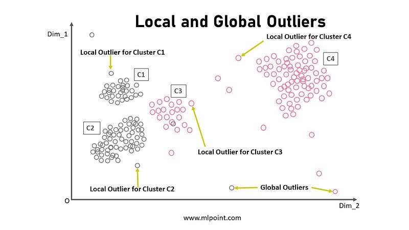
There are mainly two types of Outliers:

Global Outliers - The data points which are significantly different from the rest of the dataset are called Global Outliers.

Local Outliers -The data points which are significantly different from their neighbours in the dataset are called Local Outliers.

Detection of outliers is very important in machine learning and used in various applications such as Credit Card Fraud Detection, Cyber Security Attack, Abnormal Stock Trading e.t.c. Different methods to detect outliers are listed below:

1.Statistical-Based Outlier Detection

• Distribution-based
• Depth-based

2.Deviation-Based Outlier Detection

• Sequential exception
• OLAP data cube

3.Distance-Based Outlier Detection

• Index-based
• Nested-loop
• Cell-based
• Local-outliers

Note: Outliers should be investigated carefully as they may contain valuable information.

As the title shows, this story is about the Local Outlier Factor which is distance-based outlier detection technique where the data points lie away from a certain distance is considered as Outliers. But in the nearest neighbour algorithm, the distance threshold is replaced to assign a score to every data point to detect outlier by comparing that scores.

To understand local outlier factor in a better way please go through the given link for the basic idea of k- nearest neighbour algorithm.

Contents

1. What is the Local Outlier Factor?

2.Important parameters used for calculating Local Outlier Factors(LOF)

3.Understanding LOF with important parameters

4.Implementation using Python

5.Conclusion

6.Other sources

1. What is the Local Outlier Factor?

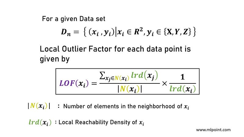
Local Outlier Factor(LOF) is an algorithm used to detect anomalous data points/outliers in any datasets. It is understood that it is used to find outliers but how. Let us understand, in this algorithm, a score (scalar value) which is called as Local Outlier Factor (LOF) is the deciding factor. The mathematical expression of finding this factor is given below-

LOF is assigned to each data points, these assigned LOF scores of each data points are compared to find outliers. The more the value of LOF of any data point more the chance that it will be an outlier.

Note: Local Outlier Factor( LOF) can be used to detect both local and global outliers.

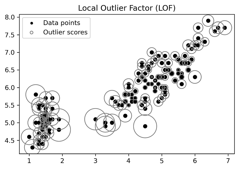
The above figure is showing LOF scores of data points with the help of circles whose radius are proportional to LOF score. The data points having Circle with a larger radius can be outliers.

2.Important parameters used for calculating Local Outlier Factors(LOF)

i) k-distance (xᵢ)

ii) Nearest Neighbor Nₖ(xᵢ)

iii) Reachability Distance (xᵢ,xⱼ)

iv) Local Reachability Density lrd( xᵢ )

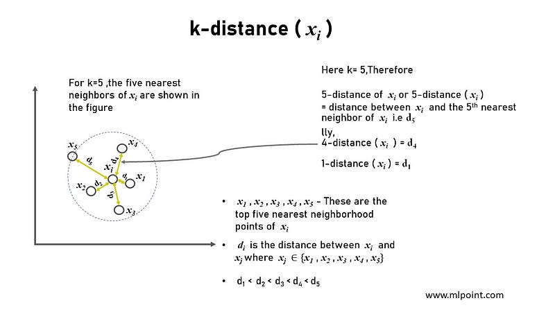
• k-distance ( xᵢ ) The k-distance of a data point xᵢ in a dataset is the distance of the kᵗʰ nearest neighbour of xᵢ from xᵢ.

• Nearest Neighbor Nₖ(xᵢ) The Nearest Neighbor of a data point xᵢ denoted by Nₖ(xᵢ) is a set of all the points that belong to the kᵗʰ nearest neighbour of xᵢ (i.e points in the neighborhood of xᵢ).

|N(xᵢ)| denotes the total number of data points present in the neighborhood of xᵢ for the given k value.

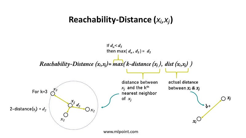
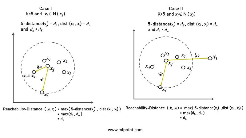
• Reachability-Distance (xᵢ,xⱼ) The Reachability-Distance of a data point xⱼ from xᵢ is the maximum of k-distance of xⱼ and the actual distance between xᵢ & xⱼ.

Mathematically,

Reachability-Distance (xᵢ,xⱼ)= max( k-distance (xⱼ ), dist (xᵢ,xⱼ) )

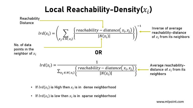
• Local Reachability Density lrd( xᵢ ) The Local Reachability Density of a data point xᵢ is the inverse of the average reachability distance of xᵢ from its neighborhood. Basically , It measures how close the neighborhood data points of xᵢ from it. The lower the density, the farther xᵢ is from its neighbours.

3.Understanding Local LOF with important parameters

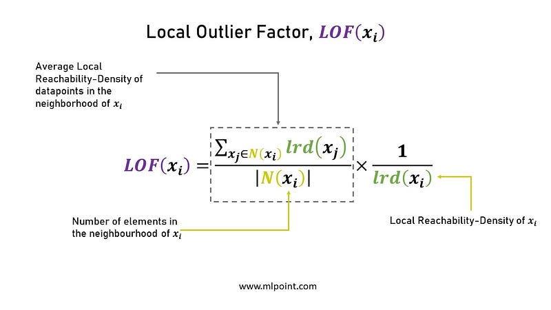
The above shows the relation between Local Reachability Density lrd( xᵢ ) and average local reachability- density of data points in the neighborhood of xᵢ.

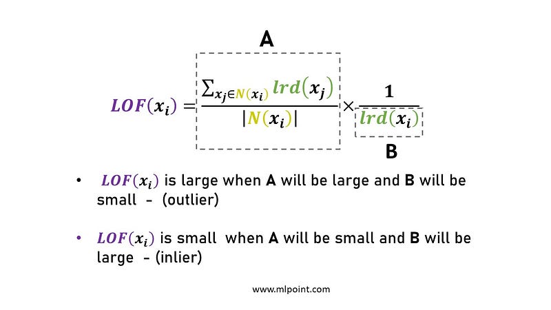
LOF(xᵢ) ~ 1 means Similar density as neighbors,

LOF(xᵢ) < 1 means Higher density than neighbors (Inlier),

LOF(xᵢ) > 1 means Lower density than neighbors (Outlier)

LOF is also called as a density-based outlier detection method because it uses the relative density of data points against its neighbors to detect outliers. As the density around the outlier is significantly different from the density of its neighbors.

4. Implementation using Python

Python has a very famous library called “sklearn” which has a good implementation of LOF.

sklearn.neighbors.LocalOutlierFactor(n_neighbors=20, *, algorithm='auto', leaf_size=30, metric='minkowski', p=2, metric_params=None, contamination='auto', novelty=False, n_jobs=None)

Let us implement local Outlier factor (LOF) algorithm on Iris Dataset:

import pandas as pd
import numpy as np
import matplotlib.pyplot as plt
import seaborn as sns
from sklearn.neighbors import LocalOutlierFactor

data = pd.read_csv("Iris_dataset.csv")

#Plotting graph between PetalLengthCm & SepalLengthCm
sns.set_style("whitegrid");
sns_plot=sns.FacetGrid(data, hue="Species", size=6,palette=['darkorange','black','red'])\
   .map(plt.scatter, "PetalLengthCm", "SepalLengthCm") \
   .add_legend();

plt.show();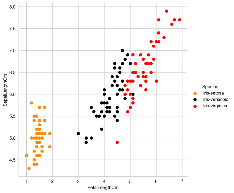

• LOF implementation on the iris dataset for k= 20 and plotting a scatter plot where LOF scores are represented with circles.

a = list(data['PetalLengthCm'])
x= np.array(a)
b = list(data['SepalLengthCm'])
y= np.array(b)
z=np.array([a,b])
X=z.T
clf = LocalOutlierFactor(n_neighbors=20, contamination=0.1)
y_pred = clf.fit_predict(X)
X_scores = clf.negative_outlier_factor_

plt.title("Local Outlier Factor (LOF)")

plt.scatter(a,b, edgecolor='grey', s=30, label='Data points',facecolors='none')

 #plotting circles with radius proportional to the outlier scores
radius = (X_scores.max() - X_scores) / (X_scores.max() - X_scores.min())

plt.scatter(a,b, s=1300 * radius, edgecolors='pink',facecolors='none', label='Outlier scores')

plt.axis('tight')
plt.xlim((0, 10))
plt.ylim((1, 10))
legend = plt.legend(loc='upper left')
legend.legendHandles[0]._sizes = [10]
legend.legendHandles[1]._sizes = [20]

plt.show()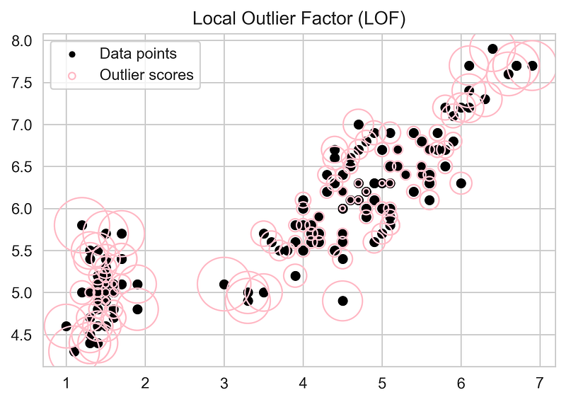

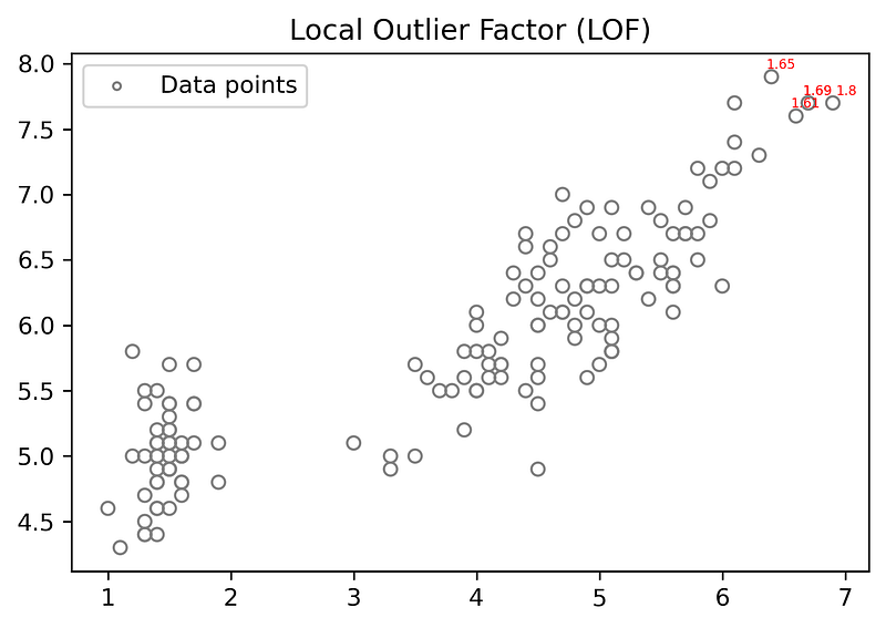
• Plotting Scatter Plot with the LOF score greater than 1.5and k= 20.

a = list(data['PetalLengthCm'])
x= np.array(a)
b = list(data['SepalLengthCm'])
y= np.array(b)
z=np.array([a,b])
X=z.T
clf = LocalOutlierFactor(n_neighbors=20, contamination=0.1)
y_pred = clf.fit_predict(X)
X_scores = clf.negative_outlier_factor_

round_off_values = np.around(X_scores, decimals =2)
new =round_off_values*(-1)

plt.title("Local Outlier Factor (LOF)")
plt.scatter(a,b, edgecolor='grey', s=30, label='Data points',facecolors='none')

for x_pos, y_pos, label in zip(x,y,new):
    if label>1.5:
        plt.annotate(label,             
                xy=(x_pos, y_pos),
                xytext=(10,5),     
                textcoords='offset points', 
                ha='right',         
                va='center',fontsize=5.5,color='r')

plt.axis('tight')
legend = plt.legend(loc='upper left')
legend.legendHandles[0]._sizes = [10]
plt.show()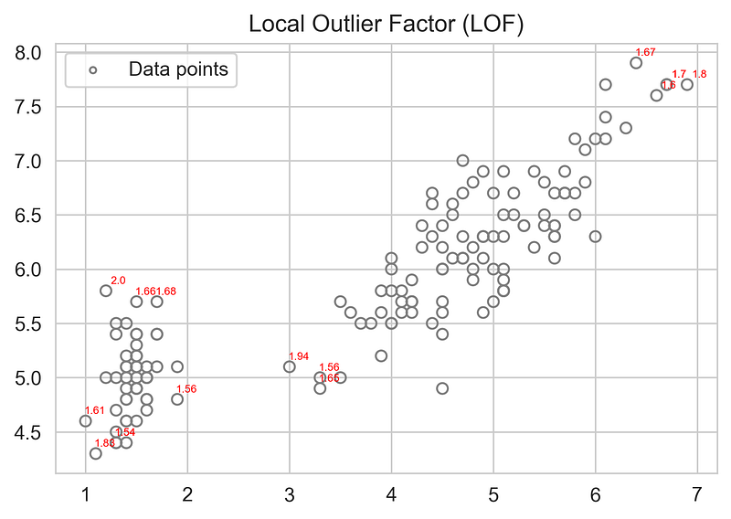

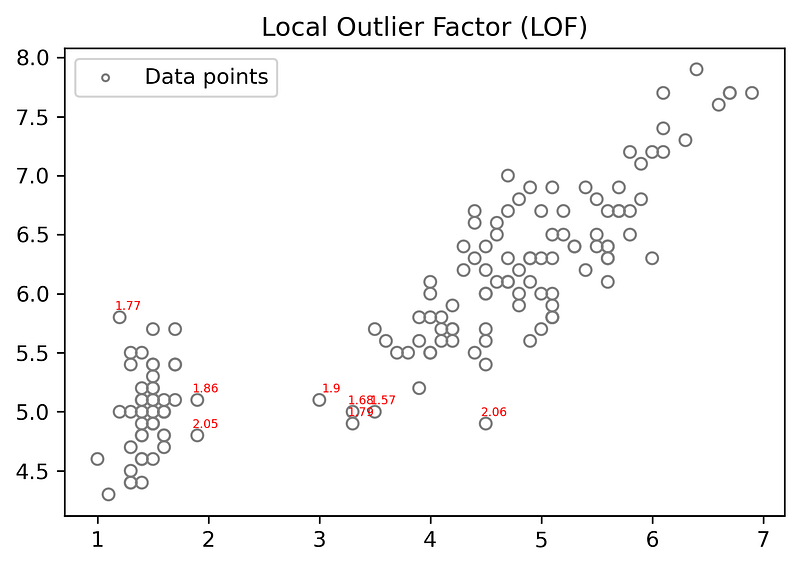
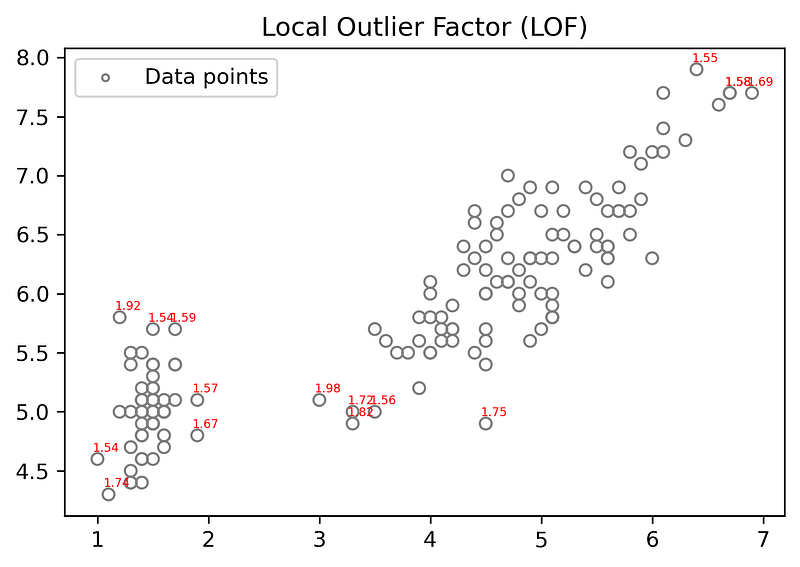
• Plotting Scatter Plot with the LOF score greater than 1.5and for k=10,k=15,k=30 and k=60.

for k=10

for k=15

for k=30

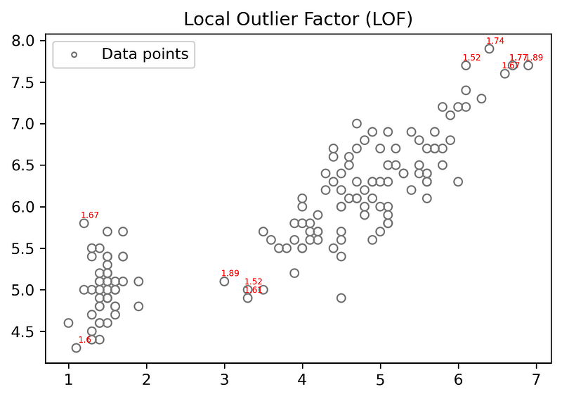
for k= 60

when k-value is high very few LOF scores are showed because at high k-value LOF of data points of local small regions are very small.

5.Conclusion The LOF of a data point gives a score by comparing the density of that point to the density of its neighbors. If the density of a point is much smaller than the densities of its neighbors (LOF ≫1), the point is far from dense areas and, hence, an outlier. Also, By varying k(n_neighbors) the outliers for the entire dataset or for the local small regions can be detected. It is not the only method for anomaly detection, there are other methods such as DBSCAN, Isolation Forests, Elliptic Envelope e.t.c.

6.Other sources: