LLM Inference Series: 5. Dissecting model performance

In the previous post, we took a deep dive into KV cache optimizations. Now we will shift gears and explore the different performance bottlenecks that can impact the speed of a machine learning model. The concepts detailed in this post apply broadly to any ML model, whether it’s used for training or inference. However, examples will focus specifically on LLM inference setups.

Before starting, let me first highly recommend this blog post [1] to which this post owes a lot.

The four kinds of performance bottlenecks

If you are unhappy with your model’s performance and ready to invest time into improvements, the first step is identifying the bottleneck type. There are four main performance bottleneck categories — three related to hardware limitations and one tied to software.

Let’s start by examining the hardware bottlenecks. Each of these corresponds to a specific operational regime:

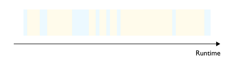
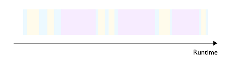
Compute bound regime: Most of the processing time, i.e. latency, is spent performing arithmetic operations (Figure 1). Compared to the other regimes and since you are primarily paying for compute, the compute bound regime is the most cost efficient and therefore the one we should aim for.

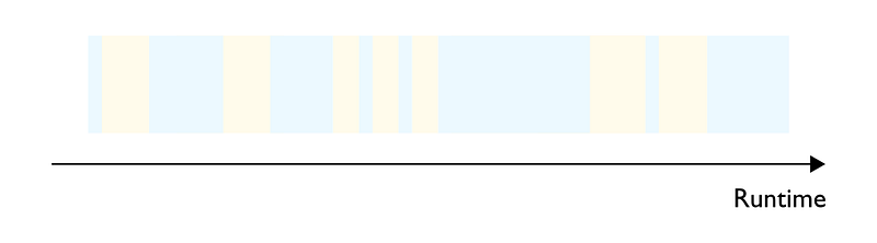
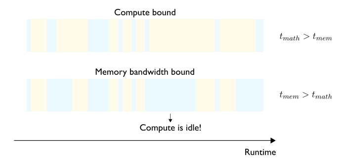
Figure 1 — A compute bound process with compute and data transfer time highlighted in yellow and blue respectively

Memory bandwidth bound: Most of the processing time is spent moving data like weight matrices, intermediate computations, etc., between chip memory and processors (Figure 2).

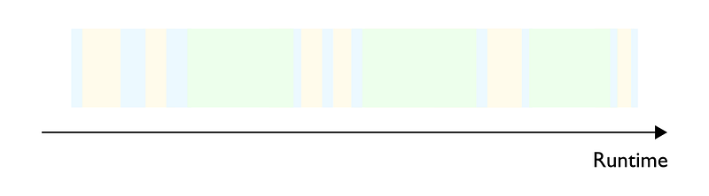
Figure 2 — A memory bandwidth bound process with compute and data transfer time highlighted in yellow and blue respectively

Communications bound (not covered by [1]): Only applies when computations and data are distributed across multiple chips. Most of the processing time is taken up by networking data transfer between chips (Figure 3).

Figure 3 — A communications bound process with compute, data transfer and network communications time highlighted in yellow, blue and green respectively

Notice: I use the word “chip” since these concepts apply to any kind of chip: CPUs, GPUs, custom silicon (Google TPUs, AWS Neuron Cores, etc.), etc.

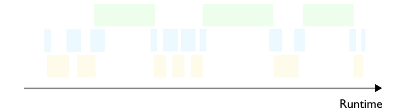
Note that modern hardware and frameworks are highly optimized and compute and data transfer tasks usually partially overlap (Figure 4). For simplicity, we will keep assuming they occur sequentially in this post.

Figure 4 — A communications bound process with overlapping data transfer

The last regime is called overhead bound and relates to software-induced limitations. In this regime, most of the processing time is spent scheduling work and submitting it to the hardware — essentially, we spend more time figuring out what to do than performing actual operations on the hardware (Figure 5). Being overhead bound is more likely when using very flexible languages (e.g. Python) or frameworks (e.g. PyTorch) that don’t require explicitly specifying all information needed at runtime (like tensor data types, target device, kernels to invoke, etc.). This missing information must be inferred at runtime, with the corresponding CPU cycles called overhead. Accelerated hardware is now so fast compared to CPUs that situations in which overhead impacts the hardware utilisation and therefore cost efficiency are likely — essentially there are times when the hardware remains idle, waiting for the software to submit the next work item.

Figure 5 — An overhead bound process with compute, data transfer and software overhead time highlighted in yellow, blue and purple respectively

Executing a model backward or forward pass involves running multiple kernel executions (~ GPU function calls). It is unlikely that all kernels operate in the same regime. What matters is identifying the regime where most of the execution time is being spent. The priority then becomes optimizing for that primary bottleneck, pinpointing the next most significant one, and so on.

Being right at identifying the type of bottleneck is critical. Each issue requires different solutions. If you get your diagnosis wrong, you may waste your time implementing an optimization that disappoints if it helps at all.

Diagnosing the limiting factor

We won’t delve into extensive detail here, but [1] highlights that when overhead bound, runtime does not scale proportionally with increased compute or data transfer. In other words, if you double your compute or data transfer capacity but runtime fails to increase accordingly, your program is likely overhead bound. Otherwise you are hardware bound, but distinguishing between bottlenecks like compute versus memory bandwidth requires access to metrics like FLOP count and data transfer volume, i.e. to use a profiler.

Bringing LLMs back into frame, keep in mind that training and inference pre-fill phase are usually compute bound while inference decoding phase is usually memory bandwidth bound on most hardwares. Optimizations primarily intended for training (e.g. lower-precision matrix multiplications) may therefore not be as helpful if applied to reduce total inference latency which is dominated by the decoding latency.

Optimizing for lower latency based on bottleneck type

Let’s look at optimizing for each type of bottleneck.

In you are in the compute bound regime, you can:

Upgrade to a more powerful and more expensive chip with higher peak FLOPS.
For particular operations like matrix multiplications, leverage specialized, faster cores like NVIDIA Tensor Cores. For example the NVIDIA H100 PCIe [2] has 51 TFLOPS peak compute using general-purpose CUDA cores vs. 378 TFLOPS with specialized Tensor Cores (in full precision).
Reduce the number of required operations. More concretely with ML models, this could mean using less parameters to achieve the same outcome. Techniques like pruning or knowledge distillation can help.
Use lower precision and faster data types for computations. For example for the same NVIDIA H100 PCIe, 8-bit Tensor Cores peak FLOPS (1 513 TFLOPS) is twice 16-bit peak FLOPS (756 TFLOPS) which is twice 32-bit peak FLOPS (378 TFLOPS). This requires quantizing all inputs however (e.g. both the weight matrices and the activations, see for example the LLM.int8() [3] or SmoothQuant [4] quantization algorithms) and using dedicated lower precision kernels.

If you are in the memory bandwidth bound regime, you can:

Upgrade to a more powerful and more expensive chip with higher memory bandwidth.
Reduce the size of the data you move using for example model compression techniques like quantization or the not-as-popular pruning and knowledge distillation. Regarding LLMs, the data size issue is mostly tackled using weight-only quantization techniques (see for example the GTPQ [5] and AWQ [6] quantization algorithms) plus KV-cache quantization.
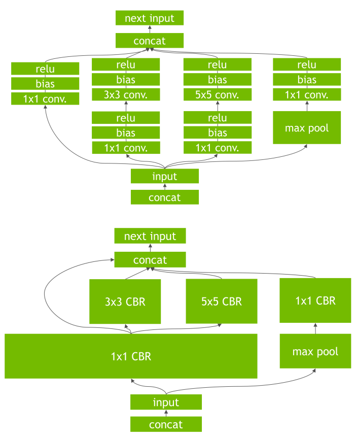
Reduce the number of memory operations. Running tasks on GPUs boils down to the execution of a directed graph of kernels (~ GPU function calls). For each kernel, inputs must be fetched from memory and outputs written to it. Fusing kernels, i.e. performing operations initially scattered across multiple kernels as a single kernel call, allows to reduce the number of memory operations. Operator fusion (Figure 6) can either be performed automatically by a compiler or manually by writing your own kernels (which is harder but necessary for complex fusions).

In the case of Transformer models, the development of highly efficient fused kernels for the attention layer remains an active field. Many optimized kernels are based on the popular FlashAttention algorithm [7]. Transformer fused kernels libraries include FlashAttention, Meta’s xFormers and the now deprecated NVIDIA FasterTransformer (merged into NVIDIA TensorRT-LLM).

Figure 6 — Example of both horizontal and vertical layer (operation) fusion applied to a CNN, inital state (above) & final state (below) [8]

If you are in the communications bound regime, you can:

Upgrade to a more powerful and more expensive chip with higher network bandwidth.
Reduce the communication volume by opting for a more efficient partitioning and collective communication strategy. For example, [9] expands the popular tensor parallelism layout for Transformer models from [10] by introducing new tensor parallel strategies that allows communication times to better scale (i.e. prevent them from becoming a bottleneck) for large chip count and/or batch sizes.

For example, the tensor parallelism layout in [10] keeps the weights shards stationary while the activation shards are moved between the chips. At the pre-fill stage and for batches of very large sequences for example, [9] notes that activations can outsize the weights. So from a communications perspective, it becomes more efficient to keep activations stationary and move weight shards instead as in their “weight-gathered” partitioning strategy.

If you are in the overhead bound regime, you can:

Trade flexibility for less overhead by using a less flexible but more efficient language like C++.
Submit kernels in groups to amortize submission overhead across multiple kernels instead of paying it per kernel. This is especially beneficial when you need to submit the same group of short-lived kernels multiple times (e.g. in iterative workloads). CUDA Graphs (integrated to PyTorch since release 1.10 [11]) serve this purpose by providing utilities to capture all GPU activities induced by a code block into a directed graph of kernel launches for one-time submission.
Extract the compute graph ahead of time (AOT) into a deployable artifact (model tracing). For example, PyTorch torch.jit.trace traces a PyTorch program and package it into a deployable TorchScript program.

You can optimize the graph further by using a model compiler.

In any case, you once again trade flexibility for less overhead since tracing/compilation requires parameters like tensors sizes, types, etc. to be static and therefore to remain the same at runtime. Control flow structures, like if-else, are also usually lost in the process.

For cases requiring flexibility incompatible with AOT compilation (e.g. dynamic tensor shapes, control flow, etc.), just-in-time (JIT) compilers come to the rescue by dynamically optimizing your model’s code right before it is executed (not as thoroughly as an AOT compiler though). For example, PyTorch 2.x features a JIT compiler named TorchDynamo. Since you don’t need to modify your PyTorch program to use it, you get the reduced overhead of using a JIT compiler while keeping the usability of the Python development experience.

Side note: Is there a difference between model optimizers and (AOT) compilers? The distinction is a bit fuzzy in my opinion. Here is how I conceptually separate the two terms.

First, both work ahead-of-time. A typical AOT compiler workflow is: trace code from a supported framework (PyTorch, TensorFlow, MXNet, etc.) to extract the compute graph into a intermediate representation (IR), apply hardware-agnostic optimizations (algebraic rewriting, loop unrolling, operator fusion, etc.) to generate an optimized graph, and finally create a deployable artifact for the target hardware including hardware-aware optimizations (selecting the most appropriate kernels, data movement optimization, etc.). Examples of AOT model compilers include PyTorch’s TorchInductor, XLA, and Meta’s Glow.

Model optimizers are tools that include AOT compilation but usually target specific hardware (e.g. Intel hardware for OpenVINO, NVIDIA hardware for TensorRT and TensorRT-LLM) and which are capable of performing additional post-training optimizations such as quantization or pruning.

Until now, we only focused on latency (time it takes to process a single request) but let’s reintroduce throughput (number of requests that can be processed per unit of time) into the frame by diving deeper into the compute and memory bandwidth bound regimes.

Bottleneck = f(Hardware, Arithmetic intensity)

Interestingly, the same algorithm processing identical inputs can be either compute bound or memory bandwidth bound, depending on the hardware used. The applicable regime is determined by the algorithm’s arithmetic intensity — the number of arithmetic operations performed per byte of memory accessed.

We want intensity values that place us in or closer to the more cost-efficient compute bound regime. As we will see, higher intensity correlates with better throughput and cost efficiency. However, some intensity drivers can degrade latency. A tradeoff between latency and throughput is nearly inevitable.

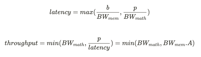
Let b be the number of bytes of data transferred to/from memory per run, and let p be the number of FLOPs (floating point operations) performed per run. Let BW_mem (in TB/s) be the hardware's memory bandwidth, and let BW_math (in TFLOPS) be the math bandwidth, also called peak FLOPS. Let t_mem be the time spent moving data bytes, and let t_math be the time spent on arithmetic operations.

Being compute bound simply means spending more time on arithmetic operations than transferring data (Figure 7).

Figure 7 — Compute vs. memory bandwidth bound regimes. Computation and data transfer times are highlighted in yellow and blue respectively.

So, we are compute bound when:

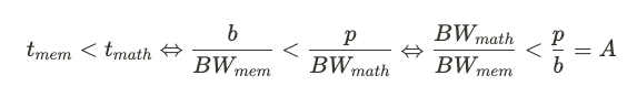
A is the algorithm’s arithmetic intensity, its dimension is FLOP per byte. The more arithmetic operations for each byte of transferred data, the higher the arithmetic intensity.

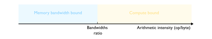
As seen in the equation, for an algorithm to be compute bound, its arithmetic intensity must exceed a hardware-dependent ratio of peak FLOPS to memory bandwidth. Conversely, being memory bandwidth bound means operating at an intensity below that same bandwidths ratio (Figure 8).

Figure 8 — The memory bandwidth / compute bound frontier

Let’s look at some real numbers for half-precision matrix multiplications (i.e. using Tensor Cores) on NVIDIA hardware (Table 1):

What does that mean? Taking the NVIDIA A10 as an example, a bandwidths ratio of 208 means moving one byte of data on that particular hardware is as fast as performing 208 FLOPs. Therefore, if an algorithm running on a NVIDIA A10 does not perform at least 208 FLOPs per byte transferred (or equivalently 416 FLOPs per half-precision number transferred), it inevitably spends more time moving data than on computations, i.e. it is memory bandwidth bound. In other words, algorithms with an arithmetic intensity below the hardware bandwidths ratio are memory bandwidth bound. QED.

Knowing that the decoding phase of the LLM inference process has low arithmetic intensity (detailed in the next blog post), it becomes memory bandwidth bound on most hardware. The NVIDIA H200 features a more favorable bandwidth ratio for such low-intensity workloads compared to the NVIDIA H100. This explains NVIDIA marketing the H200 as “supercharging generative AI inference,” as its hardware design targets this memory boundedness.

Now let’s connect the arithmetic intensity with latency and throughput:

Notice: Throughput is is expressed here in TFLOPS rather than requests per second, but both are directly proportional. Also, the fact that throughput is expressed in TFLOPS highlights its link to hardware utilization and therefore to cost efficiency. To make the link more obvious, throughput is more precisely the number of requests per chip-second, the lower the number of chip-seconds per request, i.e. the higher the throughput, the greater the cost efficiency (cf. [9] section 4).

If we plot arithmetic intensity on the x-axis and the (maximum achievable) throughput as the dependent variable on the y-axis, we get what is known as the (naive) roofline model [12] (Figure 9).

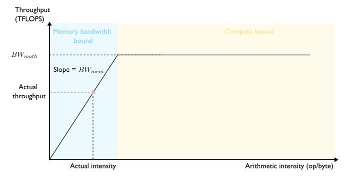
Let’s do a little thought experiment to better grasp why the throughput values on this plot are maximum achievable levels. In the compute bound regime, it is obvious: nothing prevents us from utilizing the full compute capacity, we are only bounded by the hardware’s peak capacity. In the memory bandwidth bound regime, the maximum amount of data that we can fetch in 1s is fixed by the hardware’s memory bandwidth BW_mem. Considering an algorithm of arithmetic intensity A, the maximum amount of FLOPs we can achieve in 1s is therefore BW_mem.A. CED.

What is the impact of increasing an algorithm’s arithmetic intensity? We can examine three scenarios (Figure 10):

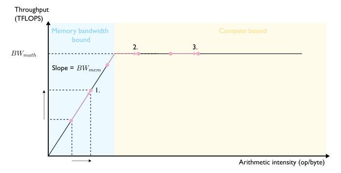
Figure 10 — Three scenarios of arithmetic intensity increase

Scenario 1: The increase in arithmetic intensity is too small to escape the memory bandwidth bound regime but involves a proportional increase in throughput. The system remains memory bandwidth bound, so the effect on latency depends on how more intensity affects data transfer for that particular algorithm.
Scenario 2: The increase in arithmetic intensity switches the system to the compute bound regime. Throughput rises to hardware peak throughput. Now compute bound, latency impact depends on how higher intensity changes total operations for that algorithm.
Scenario 3: Since already compute bound and at peak throughput, increased intensity provides no throughput gain. Latency impact still depends on how more intensity affects total computations for that algorithm.

How do we concretely increase arithmetic intensity? This depends entirely on the algorithm specifics. In the next post, we’ll examine the key parameters governing the arithmetic intensity of Transformer decoder blocks. We’ll see how raising batch size, for instance, can heighten arithmetic intensity for certain operations.

Some optimizations already discussed also boost arithmetic intensity, improving throughput and resource utilization. For Transformer models (whose decoding phase is memory bandwidth bound), arithmetic intensity is mostly improved by reducing both the number and size of data transfers via operation fusion and data (weight matrices, KV cache) quantization.

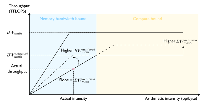
Until now, we made the crucial assumption that the algorithm implementation optimally utilizes hardware resources. For example when transferring data, the algorithm’s implementation is assumed to use 100% of the hardware’s theoretical memory bandwidth. This is obviously not the case in practice (though some implementations achieve near-optimal ressource use) so how does sub-optimal resource use impact the analysis?

It is quite simple: the bandwidth numbers above must be replaced by the actually achieved figures. The sub-optimal system lives on its own roofline curve somewhere below the optimal roofline curve (Figure 11). There are now two degrees of freedom to improve throughput: increase arithmetic intensity and/or enhance the algorithm’s implementation to better use hardware resources.

Figure 11 — Roofline model with sub-optimal resource utilization

Let’s conclude by providing a real-world example of an implementation improvement. Prior to version 2.2, the implementation of the FlashAttention kernel could become highly sub-optimal when applied to the decoding phase of inference. The previous data loading implementation made the kernel inherently less efficient at leveraging memory bandwidth in the decoding phase. Worse yet, bandwidth utilization actually further decreased with larger batch sizes; thus, performance suffered the most for longer sequences which require smaller batches due to memory limitations. The FlashAttention team addressed this issue (primarily by parallelizing data loading across the KV cache sequence length dimension) and released an optimized decoding phase kernel named FlashDecoding which achieved dramatic latency improvements for long sequence lengths [13].

Summary

In this post, we learned about the four types of bottleneck that can impact a model’s latency. Identifying the type of the main contributor to the model’s latency is critical since each type requires specific mitigation strategies.

Not considering the distributed setup for simplicity, actual hardware operations are either compute or memory bandwidth bound. The kernel’s arithmetic intensity determines the binding regime. In the lower-intensity memory bandwidth bound regime, the maximum achievable throughput is scales linearly with arithmetic intensity. In contrast, throughput is capped by peak hardware FLOPS in the compute-bound regime. Depending on the factors influencing intensity, we may be able to increase it to boost maximum throughput, potentially even reaching compute-bound performance. However, such intensity gains can adversely impact latency.

In the next blog post, we will apply this new knowledge to LLMs by taking a more detailed look at the arithmetic intensity of the Transformer decoder blocks. Stay tuned!

Change log:

02/02/2024: First release
02/02/2024: Fix error in the NVIDIA A10 example, thanks to Joaopcmoura
08/03/2024: Add additional charts

[1]: Making Deep Learning Go Brrrr From First Principles (He, 2022)

[2]: NVIDIA H100 product specifications

[3]: LLM.int8(): 8-bit Matrix Multiplication for Transformers at Scale (Dettmers et al., 2022) + GitHub repository

[4]: SmoothQuant: Accurate and Efficient Post-Training Quantization for Large Language Models (Xiao et al., 2022) + GitHub repository

[5]: GPTQ: Accurate Post-Training Quantization for Generative Pre-trained Transformers (Frantar et al., 2022) + GitHub repository

[6]: AWQ: Activation-aware Weight Quantization for LLM Compression and Acceleration (Lin et al., 2023) + GitHub repository

[7]: FlashAttention: Fast and Memory-Efficient Exact Attention with IO-Awareness (Dao et al., 2022), FlashAttention-2: Faster Attention with Better Parallelism and Work Partitioning (Dao, 2023) + GitHub repository.

[8]: Deploying Deep Neural Networks with NVIDIA TensorRT (Gray et al., 2017)

[9]: Efficiently Scaling Transformer Inference (Pope et al., 2022)

[10]: Megatron-LM: Training Multi-Billion Parameter Language Models Using Model Parallelism Shoeybi et al., 2019)

[11]: Blog post — Accelerating PyTorch with CUDA Graphs (Ngyuen et al., 2021)

[12]: Roofline: an insightful visual performance model for multicore architectures (Williams et al., 2009)

[13]: Blog post — Flash-Decoding for long-context inference (Dao et al., 2023)