Linear Regression with Gradient Descent

Understand how linear regression really works behind the scenes

It’s time to practically apply all the things that I’ve discussed so far at Data Science 365. I highly recommend you to read my previous articles published there before reading this one. Today, in this tutorial, I will discuss the most fundamental Machine Learning algorithm called Linear Regression by following the steps of the Predictive Analytics process. By the end of this tutorial, you can master the complete linear regression process from problem definition to model implementation.

Problem understanding and definition

This is the first step in the process. The goal is to understand the problem and look at it from a business perspective.

The problem is: Build a Simple Linear Regression Model to predict sales based on the money spent on TV advertising.

When we consider the model from a business perspective, it should add some value to the business in terms of money. By using the various output values of the model, the company should be able to decide whether TV advertising is effective or not and if it is effective, how much money the company should spend on TV advertising to get a particular increase in sales.

The model that I build to solve the above problem is called a Regression Model because it predicts a continuous-valued output (a classification model, by contrast, predicts a discrete-valued output — 0 or 1).

This regression model involves two variables.

• The variable that we are interested in predicting is called the target variable (=response variable/dependent variable/outcome variable). The variable sales is the target variable in our model.
• The variable that we use to predict the values of the target variable is called the explanatory variable (=feature/attribute/independent variable/predictor/regressor). The variable TV ad spending is the explanatory variable in our model.

If there is a linear relationship between the feature and the response variable, the regression model is called the linear regression model. We can confirm this by visualizing the data in a scatterplot. This will be done in the EDA section of this tutorial.

Since this linear regression model has only one feature (explanatory variable), it is called a Simple Linear Regression Model (By contrast, a multiple linear regression model uses multiple features to make a prediction). This linear regression model is also a Univariate Linear Regression Model since we are only trying to predict only one target variable (By contrast, a multivariate linear regression model predicts multiple correlated target variables).

In this tutorial, I will take a machine learning approach to linear regression. In machine learning, linear regression is a supervised learning algorithm in which you use both input and output variables to learn the mapping function from the input to the output, y=f(x). The goal is to determine the mapping function so well that when you have new input data (x), you can predict the output for that data accurately. I will discuss three different approaches to find the optimized values for the model parameters.

1. Linear Regression with Gradient Descent
2. Linear Regression with the Scikit-learn LinearRegression estimator
3. Linear Regression with the Normal Equation

In the first approach, I’ll use Python and its NumPy module along with the gradient descent algorithm to find the optimized values for the model parameters. In the second approach, I’ll use the popular Scikit-learn Machine Learning library. So, we can train the model very easily. In the third approach, I’ll use the normal equation along with the linear algebra and NumPy ndarray objects to find the optimized values for the parameters analytically.

All these algorithms end up with very similar models and make predictions in exactly the same way.

I will use the Root Mean Squared Error (RMSE) and the R-squared (R²-coefficient of determination) as the key metrics of model performance to evaluate the regression model.

I will also use various graphical techniques such as prediction error plot, residual plot and distribution of residuals to evaluate the model and verify its assumptions.

Data collection and preparation

The goal is to get a dataset that is ready for model building. Luckily, the dataset is readily available. It is in the .csv format. So, we can use the pandas read_csv() function passing the name ‘Advertising.csv’ to load the dataset. Then, we use the DataFrame head() method to see the first 5 rows of the dataset.

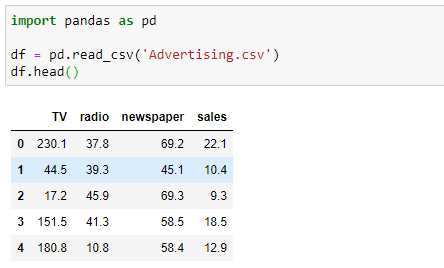
The Advertising dataset captures sales revenue generated with respect to advertisement spends across multiple channels like radio, TV and newspaper. As you can see, there are four columns in the dataset. Since our problem definition involves only sales and TV columns in the dataset, we do not need radio and newspaper columns. So, I remove the unnecessary variables in place so that the original DataFrame is modified.

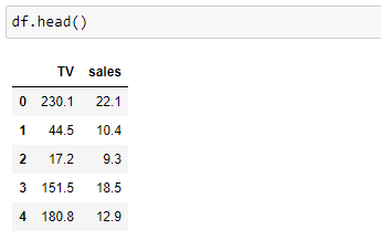
If you call the head() method again, you can see that the DataFrame (df) now consists of only TV and sales columns.

The shape of the modified advertising dataset is:

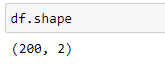
The dataset now has 2 columns and 200 rows (observations). The two columns that we’re interested in are:

• TV: the amount of money spent on TV advertising given in US dollars
• sales: the sales revenue generated with respect to advertisement spends given in 1000s of US dollars

The next step is to check the data type of each variable. For this, we can use the DataFrame info() method.

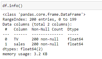
Scikit-learn machine learning library only works with numerical data types. If there are variables with string values, you need to encode them into numeric values. Fortunately, the dataset contains all numerical values so that no encoding is necessary!

Next, we need to check if there are any missing values. To do so, use the DataFrame isnull() method combined with sum().

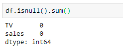
Again, the dataset is good, as it does not have any missing values!

The dataset is ready for analysis.

Dataset understanding using Exploratory Data Analysis (EDA)

The goal is to understand our dataset. The dataset is ready. It is time to apply Exploratory Data Analysis (EDA) techniques to our dataset.

EDA techniques can be divided into two types:

• Numerical techniques
• Graphical techniques

It is a good practice to use these two types of techniques simultaneously to get a better understanding of the different characteristics of our dataset and the potential relationships between the variables.

Analyze the relationship between the predictor and the target variable

For this, we can use the following techniques:

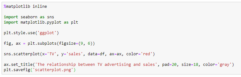
• The scatterplot
• Pearson correlation coefficient

The scatterplot is used to visualize the relationship between the predictor and the target variable. If there is a relationship between the variables, we can look for the following characteristics:

• Overall pattern: This can be a linear pattern, a curvy pattern or an exponential pattern, etc.
• Strength: This refers to how closely the points arrange.
• Direction: This can be either positive or negative. Positive means that when the predictor variable increases, the response variable also increases. Negative means that when the predictor variable increases, the response variable decreases and vice versa.

The Pearson correlation coefficient measures the strength of a linear relationship between two numerical variables. If the relationship is not linear, the correlation coefficient could be misleading. Be careful when using this! It is always a good practice to take a look at both the scatterplot and the correlation coefficient simultaneously.

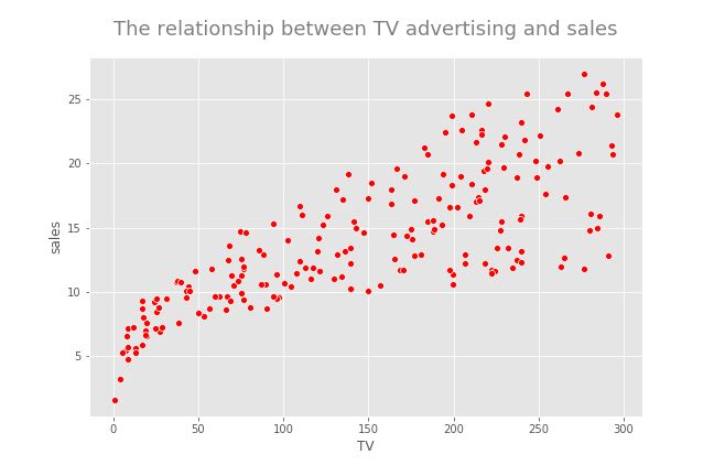
There seems to be a positive linear relationship between TV advertising and sales. Now, I calculate the Pearson correlation coefficient between the two variables to get an idea about the strength of the linear relationship.

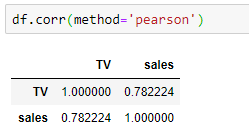
The value is approximately 0.78 which indicates that the variable TV Ad Spending is highly correlated with sales.

Since there seems to be a linear relationship between TV advertising and sales, we can build a linear regression model as our problem statement defines. What do you do if you see a non-linear relationship between the two variables? You cannot build a linear regression model. So, you may go back to step 1 and reframe the problem definition or you may stop the process by giving the reasons. But do not build a linear regression model for variables that have a non-linear relationship.

Analyze the distribution of variables

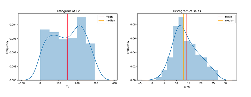
Here, we use the histogram. Now, I create two histograms for TV and sales variables in the same figure.

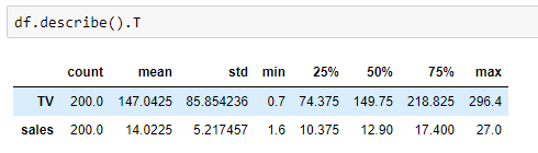
I also calculate the summary statistics for each variable with just one line of code!

Now, I interpret the above two histograms:

• Histogram of TV Ad spending: The distribution of TV Ad spending is symmetric. The mean and median are approximately the same. TV Ad spending follows a uniform distribution with a mean of 147. The center is close to 150. The typical deviation in TV Ad spending from the mean is about 85.9 units. There is a large variability in TV Ad spending. We cannot see observations outside the overall pattern.
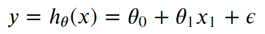
• Histogram of sales: The distribution of sales is single-peaked (unimodal) and symmetric. The mean and median are approximately the same. Sales approximately follow a normal distribution with a mean of 14.02. The center is close to 13. The typical deviation in sales from the mean is about 5.2 units. Variability in sales is not very large. There are no observations outside the overall pattern.

Now, we create boxplots. A boxplot provides a graphical representation of 5-Number Summary — MINIMUM, Q1, Median, Q3 and MAXIMUM.

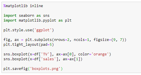
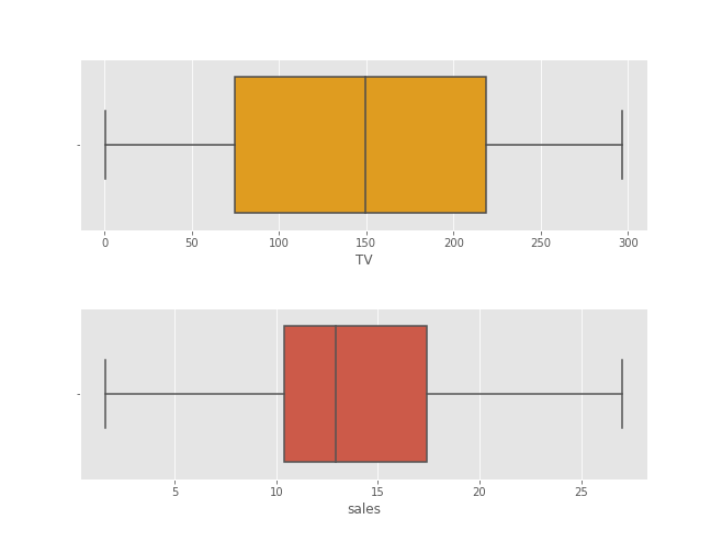
Boxplots are very useful in detecting outliers. As you can see in the above boxplots, there are no outliers present in our data. This is because there are no data points beyond the range of 1.5*IQR from Q1 and Q3.

Model building and model evaluation

The goals are to build a simple linear regression model that solves the problem, measure the model’s performance and verify the assumptions of the model.

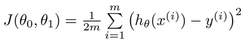
The general form for a simple linear regression model

• 𝜃0, 𝜃1: Model parameters
• y: Response variable or ℎ𝜃(𝑥): Hypothesis function
• x1: Predictor
• 𝜖: Error term (Residual)

Linear regression assumptions

• The predictors and response are linearly related — We’ve checked this assumption in the EDA section. Now, it is OK!
• The residuals (observed values-predicted values) are approximately normally distributed with the mean 0 and a fixed standard deviation — We’ll verify this assumption by drawing a histogram of residuals.
• The residuals are uncorrelated or independent — We’ll verify this assumption by drawing a residual plot.

The cost function (Mean squared error function)

• m: Number of training examples
• x(i): x-value of ith training example
• y(i): y-value of ith training example
• J(θ0​, θ1​): Cost function or mean squared error function

The goal is to minimize the above cost function so that we can find the optimized values for the model parameters. By using those values, we can fit the best possible straight line to the data.

In this tutorial, I will discuss three different approaches to find the optimized values for the model parameters.

Approach 1: Linear Regression with Gradient Descent

Here, I use Python and its NumPy module along with the gradient descent algorithm to find the optimized values for the model parameters. Here, we do not use the popular Scikit-learn Machine Learning library. So, this is a great way to have a deeper understanding of behind the scene process or the inner machinery of Linear Regression.

The gradient descent algorithm

The gradient descent algorithm is an optimization algorithm that can be used to minimize the above cost function and find the optimized values for the linear regression model parameters. For just two parameters (as in simple linear regression), the gradient descent algorithm is:

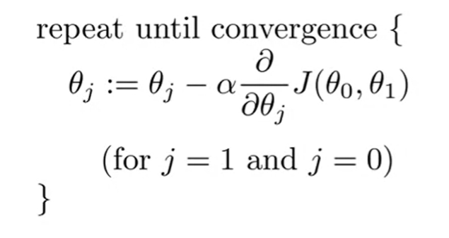
• := notation: Assignment operator. In programming, it is just = notation.
• 𝛼: Learning rate. It is a fixed value.
• Derivative term: The partial derivative of the cost function J(θ0​, θ1​) for j=0 and 1.

After we partially differentiate the cost function J(θ0​, θ1​) for j=0 and 1, the algorithm is:

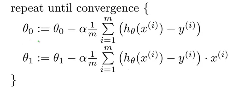
Now we follow the below steps to implement the gradient descent to our simple linear regression model.

Step 1: Start with some initial guesses for θ0​, θ1 (usually θ0​ = 0, θ1 = 0).

Step 2: Choose a good value for 𝛼.

Step 3: Simultaneously update the values of θ0​, θ1 to reduce the cost function J(θ0​, θ1​) until we hopefully end up at the minimum.

Now you may have questions like these:

• How do I choose a good value for 𝛼?
• How do I know whether the algorithm ends up at the minimum?

Choosing 𝛼 (Learning rate)

we should adjust the value of α to ensure that the gradient descent algorithm converges in a reasonable time. Failure to converge or too much time to obtain the minimum value implies that our α is wrong.

If α is too small, the gradient descent can be slow. It will require more iterations (hence time) to reach the minimum.

If α is too large, the gradient descent can overshoot the minimum. In that case, it may fail to converge or even diverge. If this happens when you run your Python code, NaN values are returned for θ0​, θ1. In that case, you should decrease the value of α and run the algorithm again.

Confirming that the algorithm ends up at the minimum

If you choose a good value for α and run the algorithm with enough iterations, the algorithm will end up at the minimum. The best way to confirm this is to plot the values of cost function over iterations of gradient descent. You should see a monotonically decreasing function (a function that is always decreasing or remaining constant and never increasing) like this:

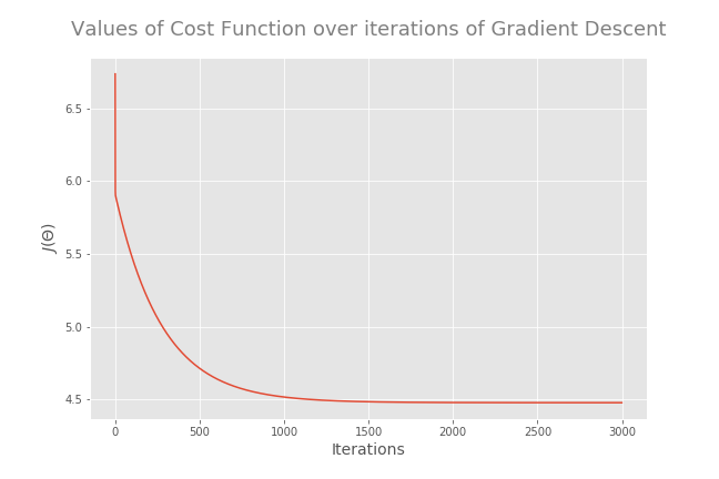
At the minimum, the derivative will always be 0 and thus the value of the cost function will not be changed. The cost at the last iteration is the minimum cost and the parameter values associated with that cost are the optimized θ values.

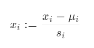
Feature scaling

If the predictors have very different scales, you must do feature scaling before running the gradient descent algorithm. If you run the algorithm without feature scaling, it will take a very long time to reach the global minimum.

• No need to do feature scaling if there is only one predictor variable.
• Do feature scaling if predictors have very different scales such as 1:100, 1:1000, etc.
• Do feature scaling only for predictors. No need to apply feature scaling for the response variable even if it has a very different scale.
• A common technique for feature scaling is mean normalization which involves subtracting the average value for an input variable and divide that result by the standard deviation of that variable.

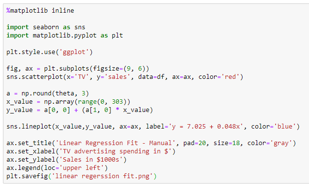
That’s it. You have just learned two algorithms in Machine Learning: Simple Linear Regression and Gradient Descent. Now, It is time to implement those algorithms to our problem by writing Python codes. Good knowledge of Python and the NumPy library is highly recommended to understand the process.

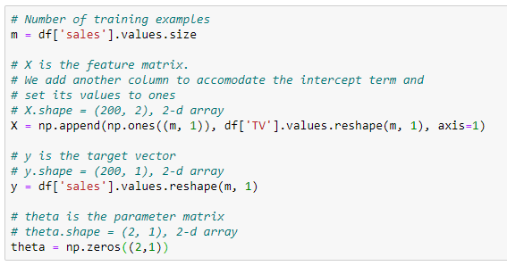
Step 1: Define X, y, theta and m

Step 2: Compute the Cost 𝐽(𝜃)

Now, I define a function called cost_function which takes the inputs X, y and theta and returns the cost.

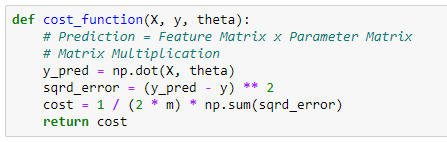
Now I calculate cost when all the parameters are zero (when parameter matrix theta contains the elements all zero).

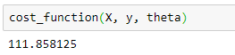
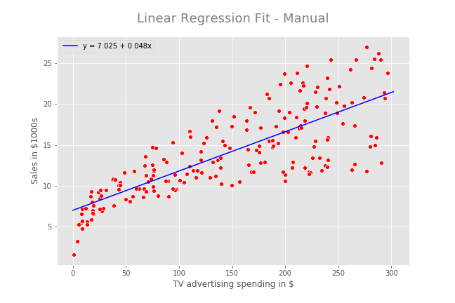
The cost is approximately 111.86. Mathematically, this is the cost associated with the line which coincides with the x-axis. This line is not the fitted regression line. From the scatterplot that I created before, the fitted regression line should have a positive slope (𝜃1 > 0). So, we can further minimize the cost by adjusting the values of model parameters.

Step 3: Run the Gradient Descent

First, I define a function called gradient_descent() which takes the inputs X, y, theta, alpha, iterations and returns the theta and costs array.

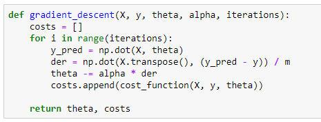
Now, I run the gradient descent.

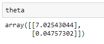
The cost associated with the above theta values is:

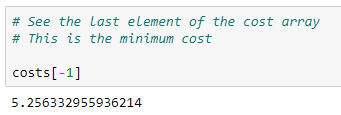
If the value of the alpha is not too high and if we run the algorithm enough iterations, the returned theta values are the optimized values for the model parameters and the last element of the returned costs array is the minimum cost. We can confirm this from a graphical visualization.

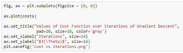
Step 4: Plot the Convergence

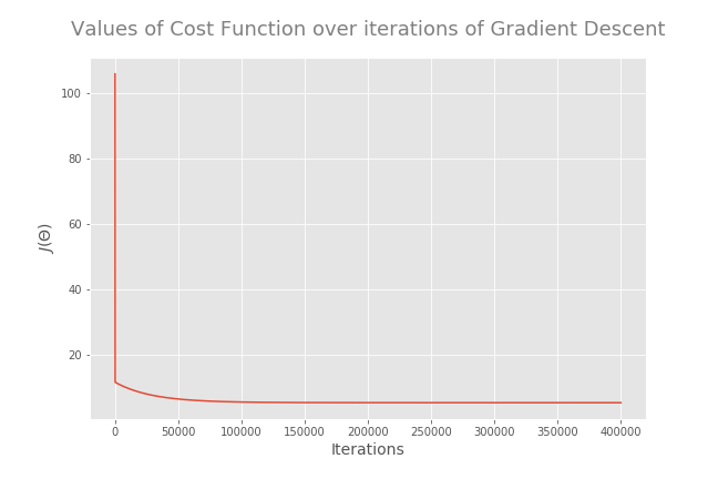
So, Gradient Descent has reached the global minimum. The returned theta values are the optimized values for the model parameters and the minimum cost (squared error) is about 5.26.

Step 5: Train the model for making predictions

Now, we can use the optimized values of theta to train the model for making predictions. First, I round the parameter values to the 3rd decimal place.

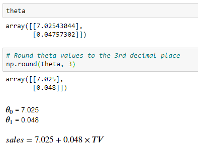
The interpretation for 𝜃1 is: For a $1 increase in TV advertising spending, the sales will increase by $48 (this is because sales are in 1000s of US dollars).

The interpretation for 𝜃0 is: Without any TV advertising spending, a particular product will have a sale of $7025 (this is because sales are in 1000s of US dollars).

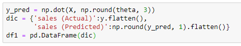
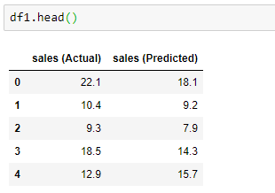
First 5 observations:

Last 5 observations:

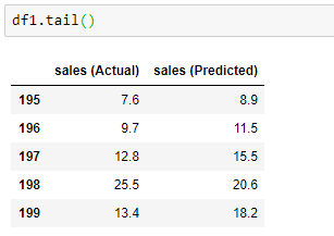
It works, although the predictions are not exactly accurate.

To make a prediction for a value that is not in our dataset, we can use the predict() function which is a user-defined function. This function is user-friendly because you need to just pass the x-value to it and the function will do the rest for you.

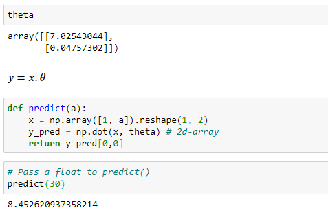
The predicted sales for the TV advertising spending of $30 is approximately 8.45 y units.

Step 6: Fit the regression line

Now, I fit the regression line manually.

Step 7: Evaluate the model performance

Now, I use the Root Mean Squared Error (RMSE) and the R-squared (R²-coefficient of determination) as the key metrics of model performance to evaluate the regression model.

With only one predictor, R² = r², where r is the Pearson correlation coefficient between sales and TV advertising.

The form for the Root Mean Squared Error (RMSE) is:

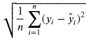
RMSE is the square root of the Mean Squared Error (MSE). The RMSE can be interpretable in y units. Smaller values for RMSE are better and the best value we can get (the perfect model) is 0.

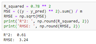
R² value is 0.61. It means that 61% of the variability observed in the sales is explained or captured by our model and the other 39% is due to some other factors. With R²=0.61, the model is not actually very good.

RMSE value is 3.24. It means that on average, the predictions of the model are 3.24 units away from the actual values. 3.24 is a better value for our model.

As a graphical method, we can use a prediction error plot to evaluate the regression model.

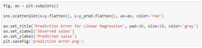
In the perfect model, all the points should be on a straight line. In general, the predictions follow the actual sales. That is good.

Step 8: Verify the assumptions

We have made some assumptions for linear regression. Now, it is time to verify them.

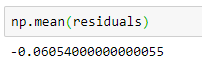
Assumption: The residuals (observed values-predicted values) are approximately normally distributed with the mean 0 and a fixed standard deviation — We’ll verify this assumption by drawing a histogram of residuals.

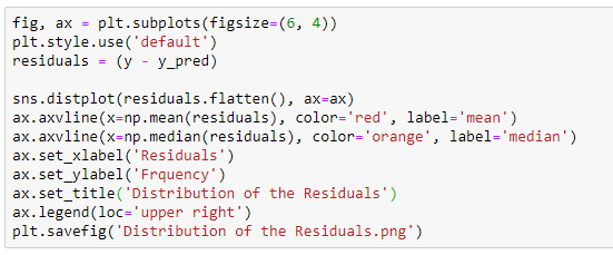
By looking at the histogram, we can verify that the residuals are approximately normally distributed with a mean of 0. The mean of the residuals is -0.061 which is very close to 0.

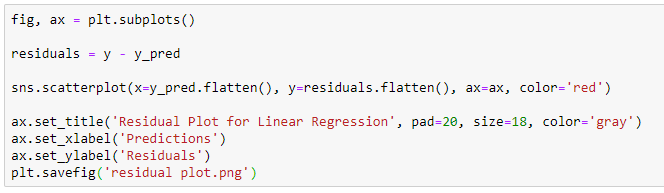
Assumption: The residuals are uncorrelated or independent — We’ll verify this assumption by drawing a residual plot.

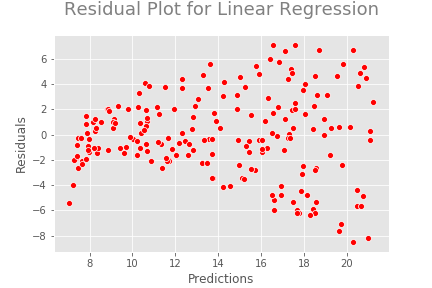
From this plot, we can clearly see some kind of non-linear pattern between predictions and residuals. Ideally, we should not see any pattern in this plot.

Approach 2: Linear Regression with the Scikit-learn LinearRegression estimator

Here we are using the popular Scikit-learn Machine Learning library. So, we can train the model very easily. The algorithm using here is Singular-Value Decomposition (SVD).

Step 1: Define X and y

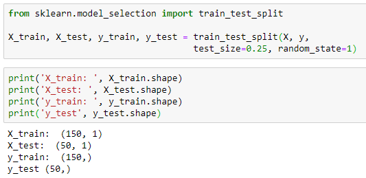
Step 2: Split the dataset into a training set and a testing set

Instead of training the model using all of the rows in the dataset, I’m going to split it into two sets, one for training and one for testing. To do so, I use the train_test_split() function (which is in the model_selection submodule in the Scikit-learn library). This function allows you to split the dataset into random train and test subsets called X_train, X_test, y_train and y_test. The following code snippet splits the dataset into a 75% training and 25% testing set. The random_state parameter of the train_test_split() function specifies the seed used by the random number generator. If this is not specified, every time you run this function you will get a different training and testing set. To get the same training and testing sets across different executions, you can specify this parameter with any integer. The popular integers are 0, 1 and 42.

Step 3: Create and fit (train) the model

Now we can create a simple linear regression model for our data. For this, we can use the Scikit-learn LinearRegression estimator. You can think of a Scikit-learn estimator as a machine learning algorithm. To build a linear regression model using this estimator, all you need to do is to create an instance of LinearRegression() class and use X_train, y_train to train the model using the fit() method of that class.

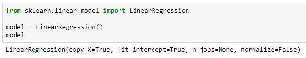
Now, the variable model is an instance of the LinearRegression() class. To train the model, we can use the fit() method of that class.

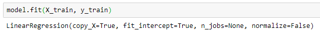
That’s it. We have just trained our model. Now, it is time to make some predictions. Before that, it is important to view the Gradient (Slope) and Intercept of the linear regression line.

Step 4: Get the Gradient and Intercept of the linear regression line

• Intercept: We use the intercept_ attribute.
• Gradient (Slope): We use the coef_ attribute.

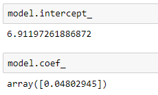
The values are slightly different from the values of the model parameters that we obtained earlier using the gradient descent algorithm.

Step 5: Make predictions

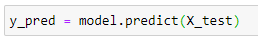
Once we have fitted (trained) the model, we can start to make predictions using the predict() method. We pass the values of X_test to this method and compare the returned (predicted) values called y_pred with y_test values.

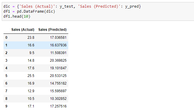
It works, although the predictions are not exactly accurate.

To make a prediction for a value that is not in our dataset, we can also use the predict() method. We pass the x-value to this method. The x-value should be in the form of a 2d array-like object such as a 2D NumPy array, a DataFrame or even a Python list of lists.

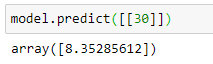
The predicted sales for the TV advertising spending of $30 is approximately 8.35 y units. We can verify the predicted value by using the linear regression formula that was given earlier:

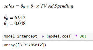
The results are exactly the same.

Step 6: Evaluate the model performance

Earlier, we calculated the Root Mean Squared Error (RMSE) and the R-squared (R²-coefficient of determination) to evaluate the regression model. Here we also calculate them but using the Scikit-learn metrics submodule.

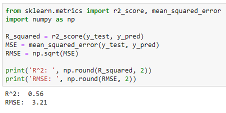
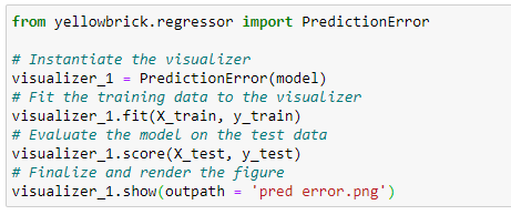
As a graphical method, we can use a prediction error plot to evaluate the regression model. This time, I use the Yellowbrick module to make the plot.

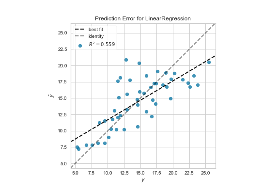
Ideally, the plot should be a straight line but for now, it is good enough. We can compare this plot against the 45-degree line, where the prediction exactly matches the model.

Step 7: Verify the assumptions

To verify the assumptions of our linear regression model, I create the histogram distribution of residuals and the residual plot in the same graph using the Yellowbrick module.

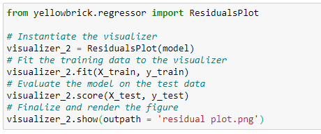
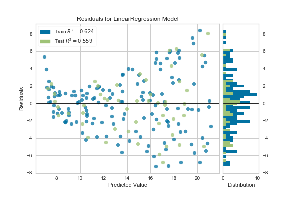
We can verify that the residuals are approximately normally distributed. But we can clearly see some kind of non-linear pattern between predictions and residuals.

Approach 3: Linear Regression with the Normal Equation

The Normal Equation

To find the value of θ that minimizes the cost function, there is a mathematical equation that gives the result directly. This is called the Normal Equation.

In this equation:

• θ: Parameter matrix which contains optimized values. It is returned as a 2d NumPy array. The shape is (n+1, 1) where n is the number of predictors.
• X: Feature matrix. It is represented as a 2d NumPy array. The shape is (m, n+1) where n is the number of predictors and m is is the number of training examples (rows/observations). The elements of the first column are all set to ones. This is to accommodate the intercept term.
• y: Target vector. It is represented as a 2d NumPy array to match the dimension. The shape is (m, 1) where m is the number of training examples (rows/observations).

Calculate optimized θ values using the normal equation

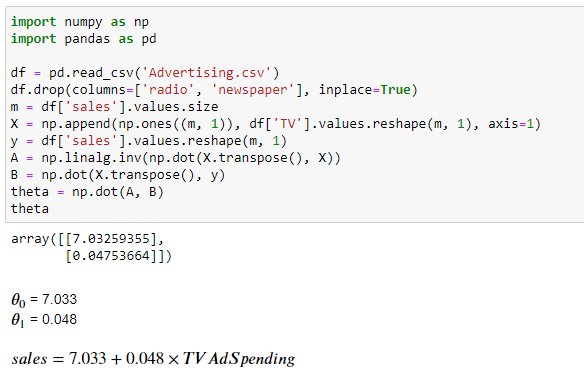
The optimized parameter values are very similar to the values obtained in approach 1 — Linear Regression with Gradient Descent.

Thanks for reading!

Special credit goes to Mick Haupt on Unsplash, who provides me with the cover image for this post.

Rukshan Pramoditha, Last edited: 2021–07–08