Analyzing the band structure of MoS2 crystal using Pylab | Towards AI

Linear Regression Analysis in Materials Sciences

Analyzing the band structure of MoS2 crystal using Pylab

This code performs linear regression on simulated band structure data for MoS2 crystal. The band structure of MoS2 was calculated in a previous article: Tutorial on Density Functional Theory using quantum espresso.

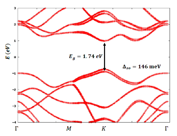
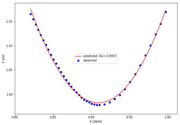
Linear regression analysis can be used to fit a parabola (degree = 2) to the conduction and valence band data in the vicinity of the K point, as shown in Figure 1. This analysis will yield important information about the electron and hole effective masses, which are key transport properties for any semiconducting material. For simplicity, we shall only focus on the conduction band.

For electron effective mass calculations, we use a quadratic (parabolic) fit (degree = 2) for our conduction band data:

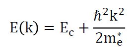
where

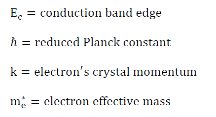
This is an example where knowledge of the behavior of the dispersion relation in the vicinity of the conduction band minimum (at K point in Figure 1) guides us to choose a quadratic fit. Even though a higher degree polynomial fit, e.g. degree = 4 produces a better accuracy (higher R-squared value), it leads to over fitting of the model, that is a model with no physical interpretation.

The data set and code for this article can be downloaded from this repository: https://github.com/bot13956/regression_band_structure.

Band Structure Analysis Using Pylab

Import Necessary Libraries

import pylab
import pandas as pd

Import Conduction Band Data

#import conduction band data: x = crystal momentum; y = energy

data=pd.read_csv('c_band.csv')

data.head(n=10)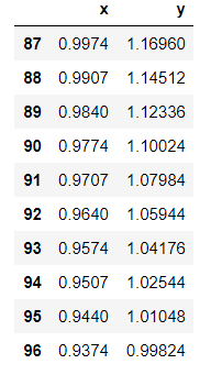

Select x Values in the Vicinity of the Conduction Band Minimum

data=data[(data.x >0.82) & (data.x<1.0)]

Perform Polynomial fit using Pylab

Xvals=data.x

Yvals=data.y

degree = 2

model=pylab.polyfit(Xvals,Yvals,degree)

estY=pylab.polyval(model,Xvals)

Calculate R-squared Value

R2 = 1 - ((Yvals-estY)**2).sum()/((Yvals-Yvals.mean())**2).sum()

Visualization of Observed and Modeled Data

pylab.figure(figsize=(10,7))

pylab.scatter(Xvals,Yvals, c='b', label='observed')

pylab.plot(Xvals,estY, c='r', label='predicted:' + ' R2' '='+ ' ' + str(round(R2,4)))

pylab.xlabel('k (2pi/a)')

pylab.ylabel('E (eV)')

pylab.xticks(pylab.arange(0.8, 1.05, 0.05))

pylab.legend(loc=10)

pylab.show()

In summary, we’ve discussed how linear regression can be used in materials sciences to analyze data generated from computational studies. We’ve seen that the primary factor in determining a good fit to any given data is the validity of the functional form to which you’re fitting. Certainly, theoretical or analytic information about the physical problem should be incorporated into the model whenever it’s available. In this example, a quadratic model was used to fit the data based on our understanding of the nearly-free electron dispersion relationship close to the conduction band minimum. This ensures that the problem of bias-variance trade-off is taken into consideration.

The data set and code for this article can be downloaded from this repository: https://github.com/bot13956/regression_band_structure.