Linear Regression

This article is about Linear regression and the different measures that determine the goodness of fit

Code for the article can be found at https://github.com/arshren/MachineLearning/blob/master/Python%20-%20Linear%20Regression%20-%20Predicting%20Temperature.ipynb

Let’s say you are concerned about climate change and wants to study the weather condition to know what parameters have an impact on the temperature.

we can use humidity, air pressure, wind speed to predict the temperature that day.

we will use linear regression here.

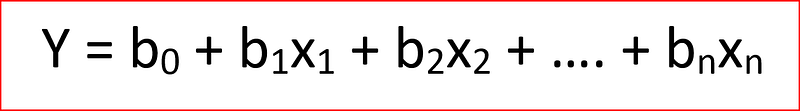
Linear regression is the simplest yet very powerful way to model linear relationship between scalar dependent and one or more independent variable.

The linear regression equation is

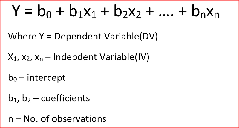
For our example, we will use the weather dataset at Kaggle -https://www.kaggle.com/budincsevity/szeged-weather

First we will import the required

import pandas as pd
import numpy as np
import seaborn as sns
import matplotlib.pyplot as plt

let’s read the data, I have downloaded my data into a folder -D:\Machine Learning — Full\Blogs dataset and renamed the file as WeatherHist.csv

weather_data = pd.read_csv("D:\Machine Learning - Full\Blogs dataset\weatherHist.csv")

Now, we want to know what are the different columns

weather_data.head(3)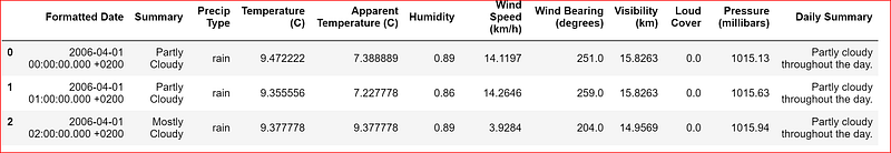

let’s explore the categorical variables in the dataset

weather_data.describe(include=['O'])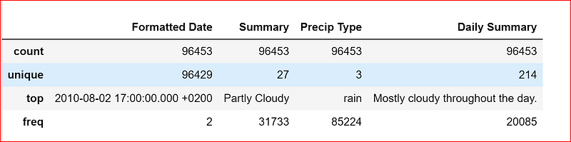

We want to predict the temperature, so let’s us find out the correlation between the different variables in the dataset

weather_data.corr()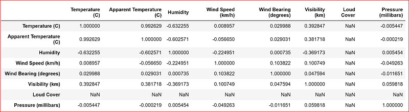

Correlation varies between +1 to -1, +1 indicates strong positive correlation, Correlation coefficient of -1 signifies perfect negative relationship, and correlation of 0 means that no relationship exists between variables

From the table above, we see strong relationship between temperature and apparent temperature, humidity and maybe we can also include visibility.

Let’s take all the relevant attributes into a new dataset and again check the correlation

data_set=weather_data.iloc[:,[0,3,4,5,8]]
data_set.corr()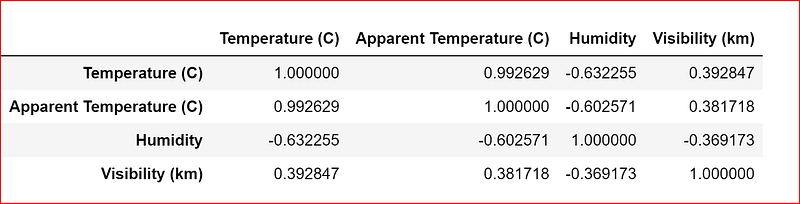

Let’s now visualize the data between temperature and other dependent variables

plotting a scatter plot between temp and humidity

sns.regplot(x=data_set["Temperature (C)"], y=data_set["Humidity"])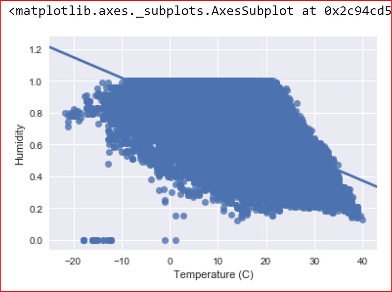

There is a negative sort of correlation between Humidity and Temperature and we also see a few outliers.

Let’s try and find the outliers so that we can remove them.

we have learnt in Inferential statistics that outliers greatly impact linear regression-POST

Below we have written a function that helps identify outliers in Humidity variable in our data set.

The way it finds outliers is based on Z score with a standard deviation greater than 3

import numpy as np
import pandas as pd
outliers=[]
def detect_outlier(data_1):
    
    threshold=3
    mean_1 = np.mean(data_1)
    std_1 =np.std(data_1)
    
    
    for y in data_1:
        z_score= (y - mean_1)/std_1 
        if np.abs(z_score) > threshold:
            outliers.append(y)
    return outliers

outlier_data = detect_outlier(data_set["Humidity"])
print (outlier_data)

we will remove these rows from the dataset to have a clean dataset for regression.

so we search for all values for Humidity in data_set with values >0.15 and create a new data set data_set_clean

data_set_clean = data_set[data_set["Humidity"]>0.15]

let’s again plot the data between Temperature and Humidity to check if we have any more outliers

sns.regplot(x=data_set_clean["Temperature (C)"], y=data_set_clean["Humidity"])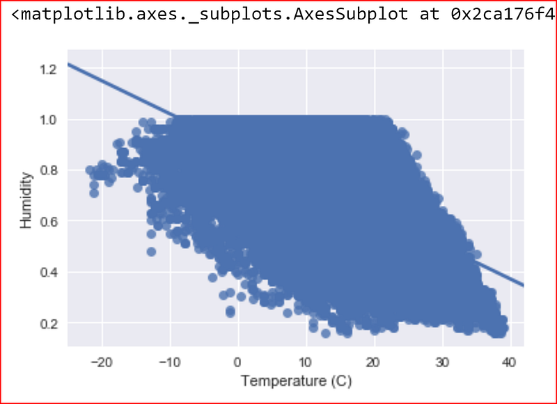

now let’s draw a scatter plot between Temp and Apparent temp

sns.regplot(x=data_set["Temperature (C)"], y=data_set["Apparent Temperature (C)"])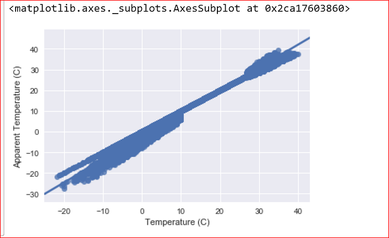

Looks like a strong positive correlation between temp and apparent temperature this seems obvious too.

we now draw a scatter plot between Temp and Visibility.

sns.regplot(x=data_set["Temperature (C)"], y=data_set["Visibility (km)"])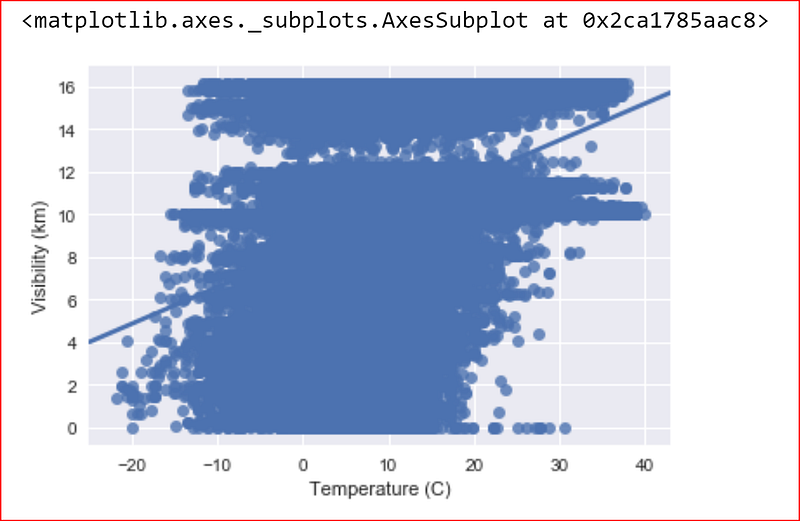

we don’t see a strong relationship between temperature and visibility so we can drop visibility.

Here X is our independent variable with Humidity and Apparent Temperature.

Y is our dependent variable with temperature that we are trying to first learn and then planning to predict

y= data_set_clean.iloc[:,[1]]
X= data_set_clean.iloc[:,[2,3]]

printing one row of X to see our independent variables

X.head(1)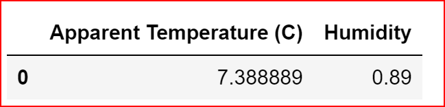

Splitting the dataset into the training set and test set with a 80:20 ratio

from sklearn.cross_validation import train_test_split
X_train, X_test, y_train, y_test = train_test_split(X, y, test_size = 0.2, random_state = 0)

we now use sklearn library for linear_models to fit our training data for Multiple Linear regression.

we import the library LinearRegression from sklearn.linear_model. Create a regressor object and then try and fit the training data

from sklearn.linear_model import LinearRegression
regressor =LinearRegression()
regressor.fit(X_train, y_train)

let’s print the different values of regressor and understand what do they mean

regressor.coef_

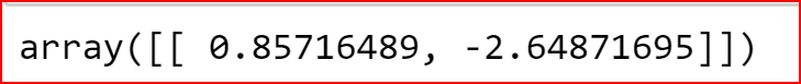
remember the Linear regression equation

• 0.857 is the b1 where x1 is apparent temperature
• -2.648 is b2 where x2 is humidity

let’s find the intercept b0

regressor.intercept_

let’s now write down the linear Regression equation for predicting temperature based on the trained dataset

temperature = 4.58 + (apparent temperature * 0.857) + (-2.648 * humidity)

we can now predict the temperature for our test dataset

y_pred = regressor.predict(X_test)

How do we know measure the fitness of our model ?

A good fitting model is one where the difference between the actual or observed values and predicted values based on the model are small and unbiased.

so if some statistics tells us that the difference between the actual and predicted values are small then we know that the model we built is a good one.

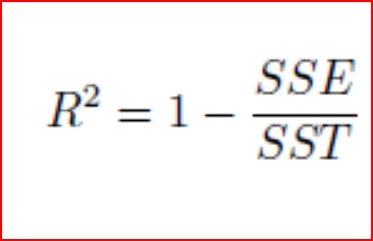
There are few statistical tools that comes to our help like coefficient of determination also called as R².

What is r-square?

It is also called as coefficient of determination.

r² gives us a measure of how well the actual outcomes are replicated by the model or the regression line. This is based on the total variation of prediction explained by the model.

R² is always between 0 and 1 or between 0% to 100%.

A value of 1 means that the model explains all the variation in predicted variable around its mean.

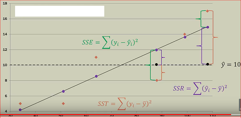
Sum square of errors(SSE) or Residuals, how far did we predict a value when compared to the actual value

SSE = Actual value -Predicted value

Sum square of total (SST), how far is the actual value when compared to the mean value

SST = Actual value -Mean value

Sum square of Regression(SSR), how far is the actual value when compared to the mean valueS

SSR = Predicted value -mean value

If the error in prediction is low then SSE will be low and r-square will be close to 1.

A caution of note here, when we add more independent variables, r² gets higher value. R² value keeps on increasing with addition of more independent variables even though they may not really have a significant impact on the predictions. This does not help us to build a good model.

To overcome this issue, we use Adjusted R². Adjusted r² penalizes the model for every addition of an insignificant independent variable.

regressor.score(X,y)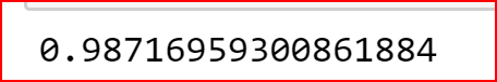

A value close to 1 for r² means a good fit.

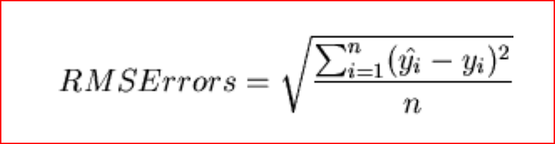
we can also calculate root mean square error also referred as RMSE.

Root Mean Square Error

shows the variation between the predicted and the actual value. since the difference between predicted and actual values can be positive and negative, to offset that difference we take the square of the difference between predicted and actual value.

Step 1: Find the difference between predicted and actual value for every observation and square the value and add them

Sum of all observation (predicted value — actual value)²

Step2: divide the sum by number of observation

Sum of all observation (predicted value — actual value)²/number of observation

Step 3: Take the square root the value from step 2

from sklearn import metrics
import math
print(math.sqrt(metrics.mean_squared_error(y_test, y_pred)))

Another library that we can use is statsmodel

import statsmodels.api as sm

In our linear regression equation x0 for the intercept is always 1. we have to explicitly create the variable x0.

ones_1 =[1] * X.count()
X["b0"]=ones_1

we now use OLS -ordinary least square to find the best fitting regression line

model = sm.OLS(y_pred,X_test).fit()

we then print the summary of the different statistics that help us evaluate our model

model.summary()

Here we get a slightly better r-square of .997 from our previous value of .987

Hope this article helped you to get a good understanding of Linear regression.