Summary

The website content explains the functionality and limitations of linear layers in neural networks, including bias, linear, and linear feed-forward layers, and emphasizes that stacking linear layers does not enhance learning capabilities.

Abstract

The article demystifies the complexity of neural networks by focusing on linear layers, which are fundamental components of these models. It breaks down the role of each type of linear layer: the bias layer learns a constant value such as an average or threshold; the linear layer learns the rate of correlation between inputs and outputs; and the linear feed-forward layer combines both functionalities to learn an offset and rate of correlation, effectively representing a line equation. The text also highlights that these layers are limited to linear relationships and that stacking them is redundant, as a single linear feed-forward layer can encapsulate the functionality of multiple linear layers. The article suggests that a linear feed-forward layer can be used for input scaling and dimensionality reduction, akin to PCA, and can even simulate scaling techniques like MinMaxScaler and StandardScaler.

Opinions

The author suggests that understanding the role of linear layers can help reduce the search space for suitable neural network architectures.
There is an opinion that trial and error, including meta-learning, is necessary for some hyper-parameter tuning, but guidelines and theories exist to assist in architecture selection.
The article posits that linear layers can learn fundamental statistical properties, such as averages and rates of change, which are essential for neural network functionality.
The author conveys that while linear layers have limitations, such as the inability to learn non-linearities, they are still valuable components of neural networks.
It is emphasized that stacking linear layers is not only unnecessary but also a waste of computational resources, as one linear feed-forward layer can represent the combined effect of multiple linear layers.

Linear layers explained in a simple way

A part of series about different types of layers in neural networks

Many people perceive Neural Networks as black magic. We all have sometimes the tendency to think that there is no rationale or logic behind the Neural Network architecture. We would like to believe that all we can do is just to try a random selection of layers, put some computational power (GPUs/TPUs) to it, and just wait, lazily.

Although there is no strong formal theory on how to select the neural network layers and configuration, and although the only way to tune some hyper-parameters is just by trial and error (meta-learning for instance), there are still some heuristics, guidelines, and theories that can still help us reduce the search space of suitable architectures considerably. In a previous blog post, we introduced the inner mechanics of neural networks. In this series of blog posts we will talk about the basic layers, their rationale, their complexity, and their computation capabilities.

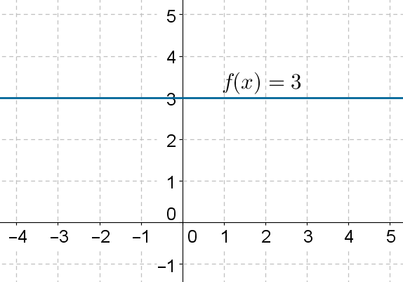
Bias layer

y = b //(Learn b)

This layer is basically learning a constant. It’s capable of learning an offset, a bias, a threshold, or a mean. If we create a neural network only from this layer and train it over a dataset, the mean square error (MSE) loss will force this layer to converge to the mean or average of the outputs.

For instance, if we have the following dataset {2,2,3,3,4,4}, and we’re forcing the neural network to compress it to a unique value b, the most logical convergence will be around the value b=3 (which is the average of the dataset to reduce the losses to the maximum. We can see that learning a constant is kind of learning a DC value component of an electric circuit, or an offset, or a ground truth to compare to. Any value above this offset will be positive, any value below it will be negative. It’s like redefining where the offset 0 should start from.

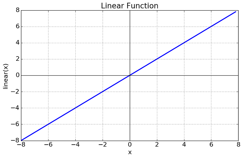
Learning a bias = learning a threshold or an average

Linear Layer

y = w*x //(Learn w)

A linear layer without a bias is capable of learning an average rate of correlation between the output and the input, for instance if x and y are positively correlated => w will be positive, if x and y are negatively correlated => w will be negative. If x and y are totally independent => w will be around 0.

Another way of perceiving this layer: Consider a new variable A=y/x. and use the “bias layer” from the previous section, as we said before, it will learn the average or the mean of A. (which is the average of output/input thus the average of the rate to which the output is changing relatively to the input).

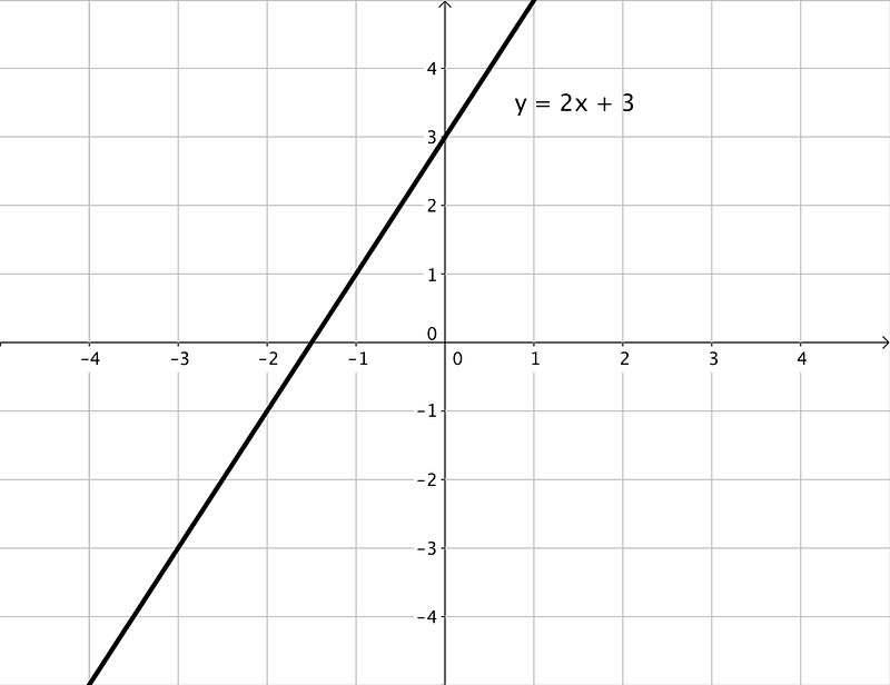
A linear curve without a bias = learning a rate of change

Linear Feed-forward layer

y = w*x + b //(Learn w, and b)

A Feed-forward layer is a combination of a linear layer and a bias. It is capable of learning an offset and a rate of correlation. Mathematically speaking, it represents an equation of a line. In term of capabilities:

This layer is able to replace both a linear layer and a bias layer.
By learning that w=0 => we can reduce this layer to a pure bias layer.
By learning that b=0 => we can reduce this layer to a pure linear layer.
A linear layer with bias can represent PCA (for dimensionality reduction). Since PCA is actually just combining linearly the inputs together.
A linear feed-forward layer can learn scaling automatically. Both a MinMaxScaler or a StandardScaler can be modeled through a linear layer.

By learning w=1/(max-min) and b=-min/(max-min) a linear feed-forward is capable of simulating a MinMaxScaler

Learning a MinMaxScaler through a linear feed-forward layer

Similarly, by learning w=1/std and b=-avg/std, a linear feed-forward is capable of simulating a StandardScaler

Learning a StandardScaler through a linear feed-forward layer

So next time, if you are not sure which scaling technique to use, consider using a feed-forward linear layer as a first layer in the architecture to scale the inputs and as a last layer to scale back the output.

A linear feed-forward. Learns the rate of change and the bias. Rate =2, Bias =3 (here)

Limitations of linear layers

These three types of linear layer can only learn linear relations. They are totally incapable of learning any non-linearity (obviously).
Stacking these layers immediately one after each other is totally pointless and a good waste of computational resources, here is why:

If we consider 2 consecutive linear feed-forward layers y₁ and y₂:

Stacking several linear feed-forward layers

We can re-write y₂ in the following form:

We can do similar reasoning for any number of consecutive linear layers. A single linear layer is capable of representing any consecutive number of linear layers. Basically, for example, scaling and PCA can be combined with one single linear feed-forward layer at the input.

Stacking Linear Layers is a waste of resources! It won’t add you any benefits to stack them.

If you enjoyed reading, follow us on: Facebook, Twitter, LinkedIn