Inside AI

Linear Discriminant Analysis, Explained

Intuitions, illustrations, and maths: How it’s more than a dimension reduction tool and why it’s robust for real-world applications.

Key takeaways

1. Linear discriminant analysis is not just a dimension reduction tool, but also a robust classification method.
2. With or without data normality assumption, we can arrive at the same LDA features, which explains its robustness.

Linear discriminant analysis is used as a tool for classification, dimension reduction, and data visualization. It has been around for quite some time now. Despite its simplicity, LDA often produces robust, decent, and interpretable classification results. When tackling real-world classification problems, LDA is often the benchmarking method before other more complicated and flexible ones are employed.

Two prominent examples of using LDA (and its variants) include:

• Bankruptcy prediction: Edward Altman’s 1968 model predicts the probability of company bankruptcy using trained LDA coefficients. The accuracy was between 80% and 90%, evaluated over 31 years of data.
• Facial recognition: While features learned from Principal Component Analysis (PCA) are called Eigenfaces, those learned from LDA are called Fisherfaces, named after the statistician, Sir Ronald Fisher. We explain this connection later.

This article starts by introducing the classic LDA and why it’s deeply rooted as a classification method. Next, we see the inherent dimension reduction in this method and how it leads to the reduced-rank LDA. After that, we see how Fisher masterfully arrived at the same algorithm, without assuming anything on the data. A hand-written digits classification problem is used to illustrate the performance of the LDA. The merits and disadvantages of the method are summarized in the end.

This article is adapted from one of my blog posts. If you prefer LaTex-formatted maths and HTML style pages, you can read this article on my blog. Also, there’s a set of corresponding slides where I present roughly the same materials, but with less explanation.

Classification by discriminant analysis

Let’s see how LDA can be derived as a supervised classification method. Consider a generic classification problem: A random variable X comes from one of K classes, with some class-specific probability densities f(x). A discriminant rule tries to divide the data space into K disjoint regions that represent all the classes (imagine the boxes on a chessboard). With these regions, classification by discriminant analysis simply means that we allocate x to class j if x is in region j. The question is then, how do we know which region the data x falls in? Naturally, We can follow two allocation rules:

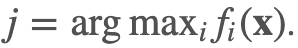
• Maximum likelihood rule: If we assume that each class could occur with equal probability, then allocate x to class j if

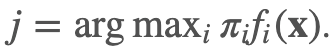
• Bayesian rule: If we know the class prior probabilities, π, then allocate x to class j if

Linear and quadratic discriminant analysis

If we assume data comes from multivariate Gaussian distribution, i.e. the distribution of X can be characterized by its mean (μ) and covariance (Σ), explicit forms of the above allocation rules can be obtained. Following the Bayesian rule, we classify the data x to class j if it has the highest likelihood among all K classes for i = 1,…,K:

The above function is called the discriminant function. Note the use of log-likelihood here. In another word, the discriminant function tells us how likely data x is from each class. The decision boundary separating any two classes, k and l, therefore, is the set of x where two discriminant functions have the same value. Therefore, any data that falls on the decision boundary is equally likely from the two classes (we couldn’t decide).

LDA arises in the case where we assume equal covariance among K classes. That is, instead of one covariance matrix per class, all classes have the same covariance matrix. Then we can obtain the following discriminant function:

Notice that this is a linear function in x. Thus, the decision boundary between any pair of classes is also a linear function in x, the reason for its name: linear discriminant analysis. Without the equal covariance assumption, the quadratic term in the likelihood does not cancel out, hence the resulting discriminant function is a quadratic function in x:

In this case, the decision boundary is quadratic in x. This is known as quadratic discriminant analysis (QDA).

Which is better? LDA or QDA?

In real problems, population parameters are usually unknown and estimated from training data as the sample means and sample covariance matrices. While QDA accommodates more flexible decision boundaries compared to LDA, the number of parameters needed to be estimated also increases faster than that of LDA. For LDA, (p+1) parameters are needed to construct the discriminant function in (2). For a problem with K classes, we would only need (K-1) such discriminant functions by arbitrarily choosing one class to be the base class (subtracting the base class likelihood from all other classes). Hence, the total number of estimated parameters for LDA is (K-1)(p+1).

On the other hand, for each QDA discriminant function in (3), mean vector, covariance matrix, and class prior need to be estimated: - Mean: p - Covariance: p(p+1)/2 - Class prior: 1 Similarly, for QDA, we need to estimate (K-1){p(p+3)/2+1} parameters.

Therefore, the number of parameters estimated in LDA increases linearly with p while that of QDA increases quadratically with p. We would expect QDA to have worse performance than LDA when the problem dimension is large.

Best of two worlds? Compromise between LDA & QDA

We can find a compromise between LDA and QDA by regularizing the individual class covariance matrices. Regularization means that we put a certain restriction on the estimated parameters. In this case, we require that individual covariance matrix shrinks toward a common pooled covariance matrix through a penalty parameter, e.g., α:

The common covariance matrix can also be regularized toward an identity matrix through a penalty parameter e.g., β:

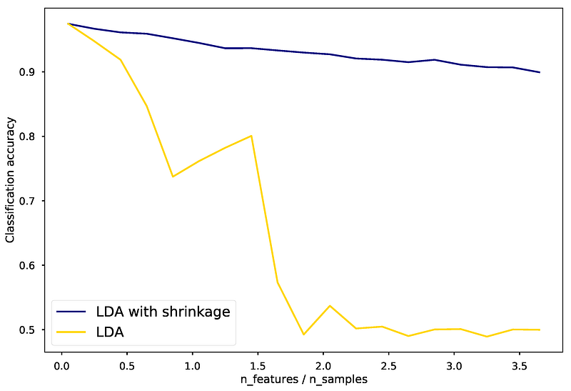
In situations where the number of input variables greatly exceeds the number of samples, the covariance matrix can be poorly estimated. Shrinkage can hopefully improve estimation and classification accuracy. This is illustrated by the figure below.

Computation for LDA

We can see from (2) and (3) that computations of discriminant functions can be simplified if we diagonalize the covariance matrices first. That is, data are transformed to have an identity covariance matrix (no correlation, variance of 1). In the case of LDA, here’s how we proceed with the computation:

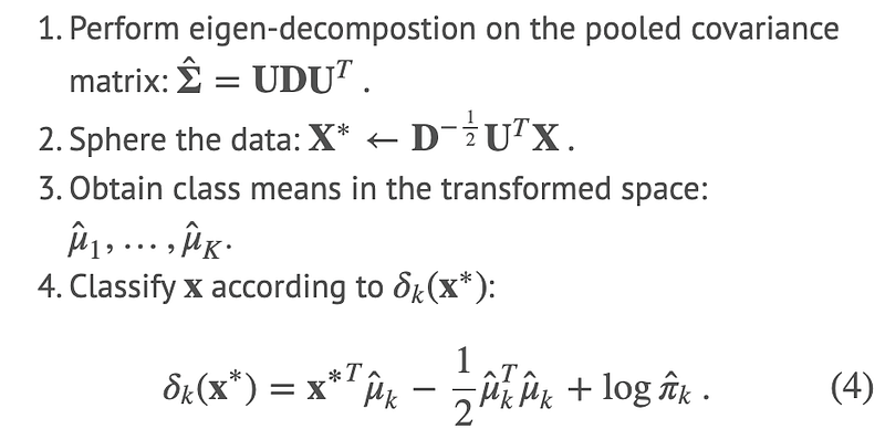
Step 2 spheres the data to produce an identity covariance matrix in the transformed space. Step 4 is obtained by following (2).

Let’s take a two-class example to see what LDA is really doing. Suppose there are two classes, k and l. We classify x to class k if

The above condition means class k is more likely to produce data x than class l. Following the four steps outlined above, we write

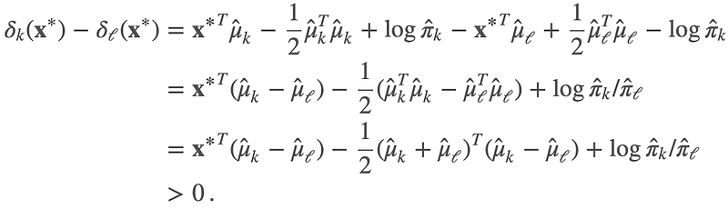
That is, we classify data x to class k if

The derived allocation rule reveals the working of LDA. The left-hand side (l.h.s.) of the equation is the length of the orthogonal projection of x* onto the line segment joining the two class means. The right-hand side is the location of the center of the segment corrected by class prior probabilities. Essentially, LDA classifies the sphered data to the closest class mean. We can make two observations here:

1. The decision point deviates from the middle point when the class prior probabilities are not the same, i.e., the boundary is pushed toward the class with a smaller prior probability.
2. Data are projected onto the space spanned by class means (the multiplication of x* and mean subtraction on the l.h.s. of the rule). Distance comparisons are then done in that space.

Reduced-rank LDA

What I’ve just described is LDA for classification. LDA is also famous for its ability to find a small number of meaningful dimensions, allowing us to visualize and tackle high-dimensional problems. What do we mean by meaningful, and how does LDA find these dimensions? We will answer these questions shortly.

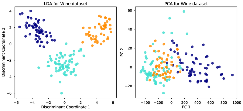
First, take a look at the below plot. For a wine classification problem with three different types of wines and 13 input variables, the plot visualizes the data in two discriminant coordinates found by LDA. In this two-dimensional space, the classes can be well-separated. In comparison, the classes are not as clearly separated using the first two principal components found by PCA.

Dimension reduction inherent in LDA

In the above wine example, a 13-dimensional problem is visualized in a 2d space. Why is this possible? This is possible because there’s an inherent dimension reduction in LDA. We have observed from the previous section that LDA makes distance comparison in the space spanned by different class means. Two distinct points lie on a 1d line; three distinct points lie on a 2d plane. Similarly, K class means lie on a hyperplane with the number of dimensions at most (K-1). In particular, the subspace spanned by the means is

When making distance comparison in this space, distances orthogonal to this subspace would add no information since they contribute equally for each class. Hence, by restricting distance comparisons to this subspace only would not lose any information useful for LDA classification. That means, we can safely transform our task from a p-dimensional problem to a (K-1)-dimensional problem by an orthogonal projection of the data onto this subspace. When p is much larger than K, this is a considerable drop in the number of dimensions.

What if we want to reduce the dimension further from p to L, e.g. two dimensional with L = 2? We can try to construct an L-dimensional subspace from the (K-1)-dimensional space and this subspace is optimal, in some sense, for LDA classification.

What would be the optimal subspace?

Fisher proposes that the much smaller L-dimensional subspace is optimal when the class means of sphered data in that space have maximum separation in terms of variance. Following this definition, optimal subspace coordinates are simply found by doing PCA on sphered class means, since PCA finds the direction of maximal variance. The computation steps are summarized below:

Through this procedure, we replace our data from X to Z and reduce the problem dimension from p to L. Discriminant coordinate 1 and 2 in the previous wine plot are found through this procedure by setting L = 2. Repeating the previous LDA procedures for classification using the new data is called the reduced-rank LDA.

Fisher’s LDA

If the derivation of the previous reduced-rank LDA looks very different from what you’ve known before, you are not alone! Here comes the revelation. Fisher derived the computation steps according to his optimality definition in a different way¹. His steps of performing the reduced-rank LDA would later be known as the Fisher’s discriminant analysis.

Fisher does not make any assumptions about the distribution of the data. Instead, he tries to find a “sensible” rule so that the classification task becomes easier. In particular, Fisher finds a linear combination of the original data, where the between-class variance, B = cov(M), is maximized relative to the within-class variance, W, as defined in (6).

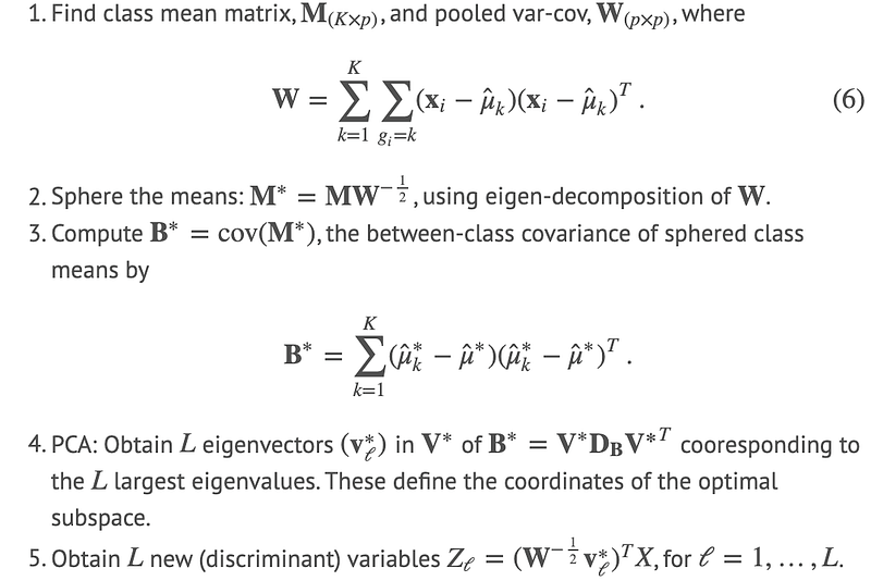
The below plot, taken from ESL², shows why this rule makes intuitive sense. The rule sets out to find a direction, a, where, after projecting the data onto that direction, class means have maximum separation between them, and each class has minimum variance within them. The projection direction found under this rule, shown in the right plot, makes classification much easier.

Finding the direction: Fisher’s way

Using Fisher’s sensible rule, finding the optimal projection direction(s) amounts to solving an optimization problem:

Recall that we want to find a direction where the between-class variance is maximized (the numerator) and the within-class variance is minimized (the denominator). This can be recast as a generalized eigenvalue problem. For those interested, you can find in my original blog post how the problem is solved.

After solving the problem, optimal subspace coordinates, also known as discriminant coordinates, are obtained as the eigenvectors of inv(W)∙B. It can be shown that these coordinates are the same as those transforming X to Z in the reduced-rank LDA formulation above.

Surprisingly, Fisher arrived at these discriminant coordinates without any Gaussian assumption on the population, unlike the reduced-rank LDA formulation. The hope is that, with this sensible rule, LDA would perform well even when the data do not follow exactly the Gaussian distribution.

Handwritten digits problem

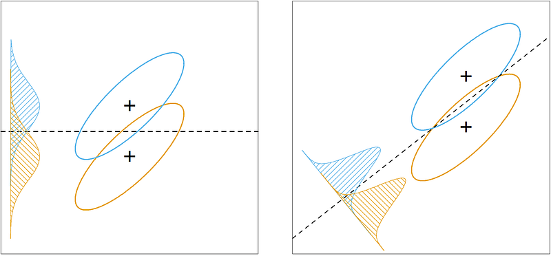
Here’s an example to show the visualization and classification ability of Fisher’s LDA, or simply LDA. We need to recognize ten different digits, i.e., 0 to 9, using 64 variables (pixel values from images). The dataset is taken from here. First, we can visualize the training images and they look like these:

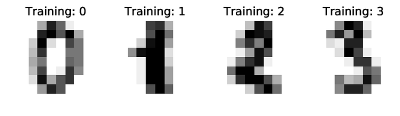
Next, we train an LDA classifier on the first half of the data. Solving the generalized eigenvalue problem mentioned previously gives us a list of optimal projection directions. In this problem, we keep the top four coordinates, and the transformed data are shown below.

The above plot allows us to interpret the trained LDA classifier. For example, coordinate 1 helps to contrast 4’s and 2/3’s while coordinate 2 contrasts 0’s and 1’s. Subsequently, coordinate 3 and 4 help to discriminate digits not well-separated in coordinate 1 and 2. We test the trained classifier using the other half of the dataset. The report below summarizes the result.

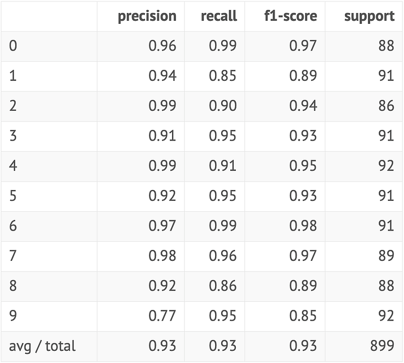
The highest precision is 99%, and the lowest is 77%, a decent result knowing that the method was proposed some 70 years ago. Besides, we have not done anything to make the procedure better for this specific problem. For example, there is collinearity in the input variables, and the shrinkage parameter might not be optimal.

Summary of LDA

Virtues of LDA:

1. Simple prototype classifier: Distance to the class mean is used, it’s simple to interpret.
2. The decision boundary is linear: It’s simple to implement and the classification is robust.
3. Dimension reduction: It provides an informative low-dimensional view on the data, which is both useful for visualization and feature engineering.

Shortcomings of LDA:

1. Linear decision boundaries may not adequately separate the classes. Support for more general boundaries is desired.
2. In a high-dimensional setting, LDA uses too many parameters. A regularized version of LDA is desired.
3. Support for more complex prototype classification is desired.

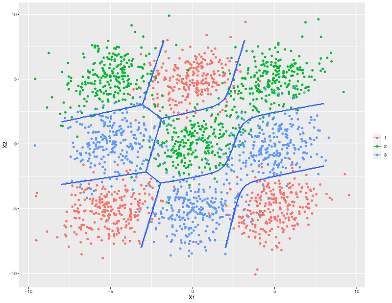
Thank you for reading until the end! In the next one, flexible, penalized, and mixture discriminant analysis will be introduced to address each of the three shortcomings of LDA. With these generalizations, LDA can take on much more difficult and complex problems, such as the one shown in the feature image.

If you are interested in more statistical learning stuff, feel free to take a look at my other articles:

References

1. R. A., Fisher, The use of multiple measurements in taxonomic problems (1936), Annals of Eugenics, 7(2), 179–188.
2. J. Friedman, T. Hastie and R. Tibshirani, The Elements Of Statistical Learning (2001), Springer Series in Statistics.
3. K. V. Mardia, J. T. Kent and J. M. Bibby, Multivariate Analysis (1979), Probability and Mathematical Statistics, Academic Press Inc.