Leveraging Value from Postal Codes, NAICS Codes, Area Codes and Other Funky-Arse Categorical Variables in Machine Learning Models

Exploiting mean/target encoding to ramp-up results.

shadgriffin/zip_code

Permalink Dismiss GitHub is home to over 50 million developers working together to host and review code, manage…

github.com

The zip (postal) code you live in says a tremendous amount about you. (At least in North America). Where you live suggests: your annual income, whether you have children, the TV shows you watch and your political leanings.

In the United States, there are over 41,000 unique zip codes. Zip codes are largely categorical. There is some broad meaning in the first two digits of the zip code. For example, Hawaii zip codes start with 9 and Maine zip codes start with 0. Beyond, very general geographic information, the codes themselves really provide little value.

What I if said that Joe lives in 76092? Does that really tell you much about him?

Not really.

Now, if I googled that zip code. I would find out that 76092 is Southlake, Texas. Southlake is one of the most affluent areas of Texas. Living in 76092 means that Joe probably makes more than 100k a year and has a college education.

My point here is that the code itself doesn’t tell us much. We have to find creative ways to extract value from the zip code.

So, given that zip codes can tell us a great deal about the people who live in them, how do we extract this information and exploit it in a machine learning model?

One way to deal with categorical variables like zip codes is to split them into dummy variables. This is what “One Hot Encoder” does. When you have a categorical variable with 41,000 unique values, dummy variables really won’t be much help, unfortunately. Using “One Hot Encoder” on zip code means you’ll create 40,999 new independent variables. Jeez, what a mess!

Another approach is something called Mean/Target Encoding. In full disclosure, I have used this technique for over twenty years, and only recently have I heard it called that. It doesn’t really matter though. Whatever you want to call it, it works quite well for categorical variables like zip code, NAICS, census block or any other meaningful categorical variable that has many distinct values.

In this example, I walk through a customer prospecting use case. The company is looking to grow its customer base but has limited marketing/sales resources. Because they don’t have enough money to contact everyone in the database, they will use a predictive model to predict those prospects most likely to acquire their product. I will not be building a model in this notebook. Rather, I will show you can leverage your historical data and zip code to create features that will build more predictive machine learning models.

As I write this, it is February 2020. So, the goal is to build a model that will predict 2020. To do this, we will use data from 2019. As we do our feature engineering, it is best not to use the same data you use for your model. Doing so leads to some major causality issues and overfitting. Instead of 2019, I will be using data from 2018 to build my features. So, just to re-cap. I will use 2018 data to build my features. Use 2019 data to build a model and apply that model to current prospects in 2020.

What if you don’t have multiple years of data? In that case, I would recommend creating a separate sample of the data set to build your features. So, as you build your model, you would split your data into four groups. This would include a Training, a Testing, a Validation and a Feature Building data set.

And finally, I will be creating summaries that are specific to a customer acquisition problem, but this technique applies to pretty much everything. For example, you could create average costs for supplier codes in health care. Or, Out of Business rates for certain NAICS codes. It is important to understand the process and realize that this technique can be applied to many different situations.

The first step is to import your python libraries.

import numpy as np
import numpy.dual as dual
import pandas as pd

As I mentioned earlier, we hope to build a model on data from 2019 to predict customer acquisition in 2020. To build our features, we will use data from 2018.

Pull in the 2018 data from Github.

!rm YEAR_2018_1.csv
!wget https://raw.githubusercontent.com/shadgriffin/zip_code/master/YEAR_2018_1.csv

!rm YEAR_2018_2.csv
!wget https://raw.githubusercontent.com/shadgriffin/zip_code/master/YEAR_2018_2.csv

pd_datax = pd.read_csv("YEAR_2018_1.csv")
pd_datay = pd.read_csv("YEAR_2018_2.csv")

df_data_1 = pd.concat([pd_datax,pd_datay])

Explore the data.

df_data_1.head()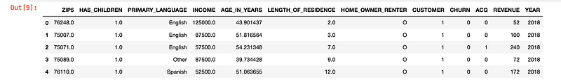

This is a fairly simple data set. Here is a description of the fields.

ZIP5 — The zip code of the individual.

HAS_CHILDREN — 1 means the individual has children. 0 means they do not.

PRIMARY_LANGUAGE — The primary language of the individual.

INCOME — Income of the individual.

AGE_IN_YEARS — Age of the individual.

LENGTH_OF_RESIDENCE — Length of time the individual has resided at their current address.

HOME_OWNER_RENTER — O means the individual owns their home.

CUSTOMER — indicates if the record belongs to a customer. 1 is a customer 0 is a non-customer.

CHURN — 1 means the individual canceled their product in 2018. 0 Means they did not cancel.

ACQ — 1 means the individual acquired the product in 2018.

REVENUE — Total Revenue of the Individual in 2018.

YEAR — the YEAR of the individual record.

It may be obvious, but the last five fields are the important ones from a feature engineering perspective. In the next few lines of code, for each zip code we will derive the following.

ZIP_PENETRATION_RATE — The percentage of individuals in a zip code who are customers.

ZIP_CHURN_RATE — the churn rate of a specific zip code

ZIP_AQC_RATE — The customer acquisition rate of the zip code.

ZIP_AVG_REV — the average revenue for customers in specific zip code.

ZIP_MEDIAN_REV — the median revenue for customers in a specific zip code

ZIP_CUSTOMERS — The total number of customers in a specific zip code.

ZIP_POPULATION — The total number of Individuals in a specific zip code.

ZIP_CHURNERS — The total number of Churners in a specific zip code.

ZIP _REVENUE — The total revenue in a specific zip code.

By creating these new fields, we can extract the value imbedded in zip code.

dfx=df_data_1

# Create churn features
zip_churn = pd.DataFrame(dfx.groupby(['ZIP5'])['CHURN'].agg(['sum']))
zip_churn['TOTAL']=dfx.CHURN.sum()

zip_churn.columns = ['ZIP_CHURNERS','TOTAL_CHURNERS']

#Create customer and popluation features
zip_cust = pd.DataFrame(dfx.groupby(['ZIP5'])['CUSTOMER'].agg(['sum','count']))
zip_cust['TOTAL_CUSTOMERS']=dfx.CUSTOMER.sum()
zip_cust['TOTAL_POPULATION']=dfx.CUSTOMER.count()

zip_cust.columns = ['ZIP_CUSTOMERS','ZIP_POPULATION','TOTAL_CUSTOMERS','TOTAL_POPULATION']

#create acquisition features
zip_acq = pd.DataFrame(dfx.groupby(['ZIP5'])['ACQ'].agg(['sum']))

zip_acq['TOTAL']=dfx.ACQ.sum()

zip_acq.columns = ['ZIP_ACQUISITIONS','TOTAL_ACQUISITIONS']

#Create Total Revenue Features
zip_rev = pd.DataFrame(dfx.groupby(['ZIP5'])['REVENUE'].agg(['sum']))
zip_rev['TOTAL']=dfx.REVENUE.sum()

zip_rev.columns = ['ZIP_REVENUE','TOTAL_REVENUE']

#create median revenue features.
df_cust=dfx[dfx['CUSTOMER']==1]

zip_med_rev = pd.DataFrame(df_cust.groupby(['ZIP5'])['REVENUE'].agg(['median']))
zip_med_rev['TOTAL']=df_cust.REVENUE.median()

zip_med_rev.columns = ['MED_REVENUE','TOTAL_MED_REVENUE']

Append the features into a single data frame.

df_18 = pd.concat([zip_cust,zip_acq, zip_churn, zip_rev,zip_med_rev], axis=1)
df_18.reset_index(level=0, inplace=True)

Note that you have to be careful of small sample sizes when calculating averages and ratios. In this example, I only calculate a rate or average for a zip code if there are more than 100 people in the zip code. You want to avoid situations where a metric is high or low only because the sample is small. For example, if you have 2 people in a zip code and one is a customer, the penetration rate would be extremely high (50%). This high number doesn’t mean that the zip code is fertile grounds for prospecting. Maybe it is. Maybe it isn’t. If you only have two people in your sample, the statistic really has no value.

Like I mentioned earlier, I only use a statistic or ratio if there are more than 100 people are in the zip code. If there is less than 100 people, I use the global average or ratio. Note that there is nothing magical about 100. You should use a number that is logical and meets the needs of your business case. I have also seen examples were people will use a weighted metric if there is a small sample size for a particular group. That is, they will take the cases in the zip code and combine with the global average/ratio in a weighted manner. I think that is a bit over-kill, but if it floats your boat, go for it.

df_18[‘ZIP_PENETRATION_RATE’] = np.where(((df_18[‘ZIP_CUSTOMERS’] <100 )), (df_18[‘TOTAL_CUSTOMERS’])/(df_18[‘TOTAL_POPULATION’]), (df_18[‘ZIP_CUSTOMERS’])/(df_18[‘ZIP_POPULATION’]))
df_18[‘ZIP_ACQ_RATE’] = np.where(((df_18[‘ZIP_CUSTOMERS’] <100 )), (df_18[‘TOTAL_ACQUISITIONS’])/(df_18[‘TOTAL_POPULATION’]), (df_18[‘ZIP_ACQUISITIONS’])/(df_18[‘ZIP_POPULATION’]))
df_18[‘ZIP_CHURN_RATE’] = np.where(((df_18[‘ZIP_CUSTOMERS’] <100 )), (df_18[‘TOTAL_CHURNERS’])/(df_18[‘TOTAL_CUSTOMERS’]), (df_18[‘ZIP_CHURNERS’])/(df_18[‘ZIP_CUSTOMERS’]))
df_18[‘ZIP_AVG_REV’] = np.where(((df_18[‘ZIP_CUSTOMERS’] <100 )), (df_18[‘TOTAL_REVENUE’])/(df_18[‘TOTAL_CUSTOMERS’]), (df_18[‘ZIP_REVENUE’])/(df_18[‘ZIP_CUSTOMERS’]))
df_18[‘ZIP_MED_REV’] = np.where(((df_18[‘ZIP_CUSTOMERS’] <100 )), (df_18[‘TOTAL_MED_REVENUE’]), (df_18[‘MED_REVENUE’]))

df_18=df_18[[‘ZIP5’, ‘ZIP_CUSTOMERS’, ‘ZIP_POPULATION’, ‘ZIP_ACQUISITIONS’, 
 ‘ZIP_CHURNERS’, ‘ZIP_REVENUE’,’ZIP_PENETRATION_RATE’,
 ‘ZIP_ACQ_RATE’, ‘ZIP_CHURN_RATE’, ‘ZIP_AVG_REV’, ‘ZIP_MED_REV’]]

df_18.head()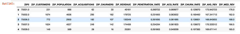

It is easy to get lost in python code, but let’s take a step back and remember our objective. Our objective is to extract the hidden value inside a categorical variable with 41000 unique values. That is, make a variable useful when the actual values of the variable are not useful. This is what we have done. For example, the value 75001 is not very useful. Knowing, however, that the zip code 75001 has a product penetration rate of .260722 is very useful.

Now that we have created out zip code level features, we can append them to our modeling data set, 2019 data.

Collect the data from GitHub. And append the features to the 2019 data.

!rm YEAR_2019.csv
!wget https://raw.githubusercontent.com/shadgriffin/zip_code/master/YEAR_2019.csv
df_2019 = pd.read_csv("YEAR_2019.csv")

df_2019 = pd.merge(df_2019, df_18, how='inner', on=['ZIP5'])

df_2019.head()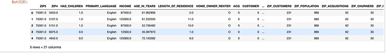

Now we can use our features to build an Acquisition Model using ACQ as a dependent variable. The features should allow us to extract the full predictive value from the zip code field.

One last note. When you actually deploy the model to our 2020 data, use the 2019 data to create your zip code feature variables, not 2018. This makes sense right? The features are extracted from the previous year of data. When we build a model for 2019, this was 2018. When we deploy the model for 2020, this would be 2019.

I hope this was helpful.