Let’s stop being gullible. You can’t predict stocks with a simple LSTM.

Dear Medium reader, Like many of us, I began my journey into algorithmic trading with stars in my eyes. It was through articles and catchy headlines that I was able to believe for a moment that predicting the stock market was child’s play. Who wouldn’t be tempted to try it when you read this kind of headline on serious forums: “Predict the stock market with AI and LSTM”.

Today, in my new article, we’re going to demonstrate in practical terms (and with a sense of humour!) that this is obviously not viable!

0. Imports

To carry out our study, we will use the following libraries:

import math
import json
import numpy as np
import pandas as pd
import requests
from sklearn.preprocessing import MinMaxScaler 
import matplotlib.pyplot as plt
from sklearn.model_selection import train_test_split
import tensorflow as tf
from tensorflow import keras
from tensorflow.keras import layers
from keras.utils.vis_utils import plot_model

1. Collecting data

For the purposes of this study, we’re going to look at some of the stock prices most commonly used by this type of author. Of course, we won’t be basing our analysis on a **share that’s made you laugh** or Gamestop, but on a stock that makes you dream, like AAPL, MSFT or many others. It’s certain that if you want to sell dreams, it’s easier to base yourself on stocks like these.

To retrieve this data, we’re going to use Alpaca Market, a company dedicated to algorithmic traders, whether professional or not, which enables us to implement real investment solutions.

def get_historical_prices(symbols, interval = '1Day', start_date = None):
    
    
    def fetch(url, next_page_token = None):
        
        if next_page_token:
            url+=f'&page_token={next_page_token}'
            
        headers = {
            "accept": "application/json",
            "APCA-API-KEY-ID": "YOUR-API-KEY",
            "APCA-API-SECRET-KEY": "YOUR-API-SECRET-KEY"
        }

        response = requests.get(url, headers=headers, verify=False)

        data = json.loads(response.text)
        try:
            next_page_token = 'stop' if str(data['next_page_token']) == 'None' else str(data['next_page_token'])
        except:
            next_page_token = 'stop'
        
        return data['bars'], next_page_token
    
    if start_date:
        url = f"https://data.alpaca.markets/v2/stocks/bars?symbols={'%2C'.join(symbols)}&timeframe={interval}&start={start_date}&limit=10000&adjustment=raw&feed=iex"
    else:
        url = f"https://data.alpaca.markets/v2/stocks/bars?symbols={'%2C'.join(symbols)}&timeframe={interval}&limit=10000&adjustment=raw&feed=iex"

    historical_prices = {}
    
    next_page_token = None
    while next_page_token != 'stop':
        data, next_page_token = fetch(url, next_page_token)
        print(next_page_token)
        historical_prices.update(data)
    
    print(historical_prices)
    print('Data Downloaded')
    
    prices = [[[dict['t'],dict['c']] for dict in historical_prices[symbol]] for symbol in symbols]
    
    active_symbols = []
    stocks = {}
    for i in range(len(symbols)):
        try:
            stocks[symbols[i]] = pd.DataFrame(prices[i], columns=['date', 'close']).sort_values(by='date', ascending=True)
            active_symbols.append(symbols[i])
        except:
            print('bug with: ', symbols[i])
            
    return stocks, list(stocks.keys())

# Download data
symbols = ['MSFT']
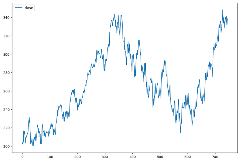
stocks, symbols = get_historical_prices(symbols, interval='1Day', start_date='2020-09-01')
stocks

Let’s plot the MSFT share price to show these newcomers what we’re all about.

2. Setting the LSTM

(This part is just to set the LSTM for a newcomer, if you are at ease with basics LSTM, go directly to section 3.)

No more daydreaming, it’s time to code! Let’s implement our LSTM in the best possible way, with a little pre-processing.

First of all, we’re going to scale the data

# Define the dataframe, here we’re looking at MSFT
df = stocks['MSFT'][['date', 'close']]


# Scaling the data
scaler = MinMaxScaler(feature_range=(0,1))
scaled_values = scaler.fit_transform(np.array(df.sort_values(by='date', ascending=True)['close']).reshape(-1,1))

scaled_df = df.copy()
scaled_df['close'] = scaled_values
scaled_df

Then split them into two parts. One for training and one for testing. (be careful to set shuffle=False, as our data must be in chronological order).

train_df, test_df = train_test_split(scaled_df, test_size=0.2, shuffle=False)
train_df

Let’s set up the rolling windows for the LSTM.

# Set up the train rolling window for the LSTM
x_train = []
y_train = []

for i in range(30, len(train_df)):
    x_train.append(train_df.iloc[i-30:i]['close'])
    y_train.append(train_df.iloc[i]['close'])
    
x_train, y_train = np.array(x_train), np.array(y_train)
x_train = np.reshape(x_train, (x_train.shape[0], x_train.shape[1], 1))

# Set up the test rolling window for the LSTM
x_test = []
y_test = []

for i in range(30, len(test_df)):
    x_test.append(test_df.iloc[i-30:i]['close'])
    y_test.append(test_df.iloc[i]['close'])

x_test = np.array(x_test)
x_test = np.reshape(x_test, (x_test.shape[0], x_test.shape[1], 1))

Now it’s time to build our LSTM architecture. To do this, we’ll adopt the most basic version possible.

model = keras.Sequential()
model.add(layers.LSTM(128, return_sequences=True, input_shape=(x_train.shape[1], 1)))
model.add(layers.LSTM(64, return_sequences=False))
model.add(layers.Dense(32))
model.add(layers.Dense(1))
model.summary()

And finally, let’s train our AI.

model.compile(optimizer='adam', loss='mean_squared_error')
model.fit(x_train, y_train, batch_size= 1, epochs=3)

3. A first prediction

Using our LSTM, let’s predict the test values and look at the fabulous result we get.

predictions = model.predict(x_test)
predictions = scaler.inverse_transform(predictions)
validation = test_df[30:].copy()
validation['predictions'] = predictions
plt.figure(figsize=(16,8))
plt.title('Model')
plt.xlabel('Date')
plt.ylabel('Close Price USD ($)')
plt.plot(df['close'])
plt.plot(validation[['predictions']])
plt.legend(['Base', 'Predictions'], loc='lower right')
plt.show()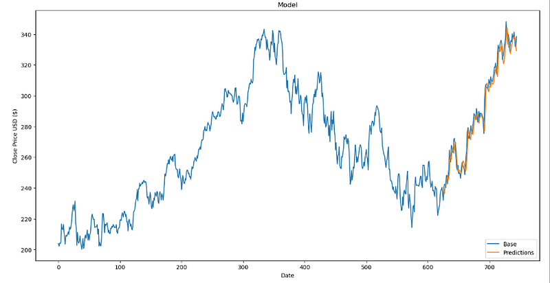

INCREDIBLE!!! Our prediction fits the curve perfectly.

This is where the beginner will be fooled. It’s all very well to stop your article here and get thousands of views, but there’s something I feel needs to be made clear…

For each prediction, the LSTM uses the last 30 values (in our situation). These last 30 values are true and not predicted… We don’t make predictions based on predictions. In other words, we only forecast 1 day in advance.

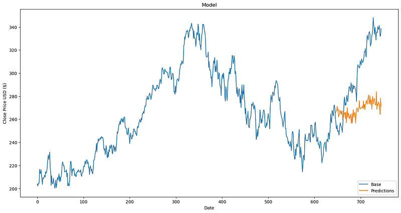
3. Back to reality

If we want to predict in the long term, we base our prediction on predictions etc. The errors then multiply at breakneck speed! Now let’s simulate this on python by removing the first value of X test and adding the last position of the predicted value, etc etc.

import numpy as np
import pandas as pd
from tqdm import trange
from sklearn.preprocessing import MinMaxScaler
from keras.models import Sequential
from keras.layers import LSTM, Dense

# Create a time series
df_train = df.iloc[:-100].copy()
time_series = np.array(df_train['close'])

# Normalization
scaler = MinMaxScaler(feature_range=(0, 1))
normalized_series = scaler.fit_transform(time_series.reshape(-1, 1))

# Training data
lookback = 30
X_train, y_train = [], []
for i in range(len(normalized_series) - lookback):
    X_train.append(normalized_series[i:i+lookback, 0])
    y_train.append(normalized_series[i+lookback, 0])
X_train, y_train = np.array(X_train), np.array(y_train)
X_train = np.reshape(X_train, (X_train.shape[0], X_train.shape[1], 1))

# Test data
last_instances = normalized_series[-lookback:]
X_test = np.array([last_instances])
X_test = np.reshape(X_test, (X_test.shape[0], X_test.shape[1], 1))

# Prediction
predicted_values = []

for i in trange(100):
    model = Sequential()
    model.add(LSTM(128, input_shape=(lookback, 1)))
    model.add(Dense(32,activation='relu'))
    model.add(Dense(1,activation='sigmoid'))
    model.compile(loss='mean_squared_error', optimizer='adam')
    model.fit(X_train, y_train, epochs=1, batch_size=1, verbose=0)
    predicted_value = model.predict(X_test)
    X_test = np.reshape(np.array([np.concatenate((X_test.reshape(lookback,)[1:], predicted_value[0])).reshape(-1, 1)]), (X_test.shape[0], X_test.shape[1], 1))
    predicted_values.append(scaler.inverse_transform(predicted_value)[0][0])

print("Predicted values:", predicted_values)

Now let’s take a look at the result with a long-term prediction and how quickly it deviates from reality.

4. Conclusion

To conclude, these headlines are very catchy and allow these authors to get a lot of views, but they are misleading and only show part of the truth. Nevertheless, it still allows people to think a little about these technologies and arouses their curiosity, we can’t take that away from them!

However, LSTMs should not be thrown away, because they are good indicators of the next value to be predicted! We’ll be talking about them in a future series of articles on long-short equity trading strategies! Thank you for your time and take care!

PS : A bonus part has been added at the end

5. Bitcoin

Previously in this article, we worked on shares of the stock market but after consideration, I think that would be worth it to also test it on the bitcoin. Please find below a slightly different function to get the historical data from Alpaca (no need Api Key for the bitcoin). And also different results ! (No others changes are needed)

def get_historical_prices(symbols, interval = '1Day', start_date = None):
    
    def fetch(url, next_page_token = None):
        
        if next_page_token:
            url+=f'&page_token={next_page_token}'

        response = requests.get(url, verify=False)

        data = json.loads(response.text)
        try:
            next_page_token = 'stop' if str(data['next_page_token']) == 'None' else str(data['next_page_token'])
        except:
            next_page_token = 'stop'
        
        return data['bars'], next_page_token
    
    if start_date:
        url = f"https://data.alpaca.markets/v1beta3/crypto/us/bars?symbols={'%2C'.join(symbols)}&timeframe={interval}&start={start_date}&limit=10000"
    else:
        url = f"https://data.alpaca.markets/v1beta3/crypto/us/bars?symbols={'%2C'.join(symbols)}&timeframe={interval}&limit=10000"

    historical_prices = {}
    
    next_page_token = None
    while next_page_token != 'stop':
        data, next_page_token = fetch(url, next_page_token)
        print(next_page_token)
        historical_prices.update(data)
    
    print(historical_prices)
    print('Data Downloaded')
    
    prices = [[[dict['t'],dict['c']] for dict in historical_prices[symbol]] for symbol in symbols]
    
    active_symbols = []
    stocks = {}
    for i in range(len(symbols)):
        try:
            stocks[symbols[i]] = pd.DataFrame(prices[i], columns=['date', 'close']).sort_values(by='date', ascending=True)
            active_symbols.append(symbols[i])
        except:
            print('bug with: ', symbols[i])
            
    return stocks, list(stocks.keys())

symbols = ['BTC/USD']
stocks, symbols = get_historical_prices(symbols, interval='1Day', start_date='2016-01-01')
df = stocks['BTC/USD'][['date', 'close']]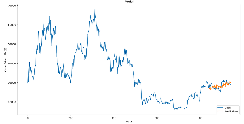

Ouch… As beautiful as it can be, I dare you to bet even 1k£ on such a prediction…

6. Alternative algorithm but faster

As you may have noticed, I have trained the LSTM in every loop which considerably reduced the speed of the LSTM but produced much more convincing results. Below is a much faster but less accurate code, as you will see.

import numpy as np
import pandas as pd
from sklearn.preprocessing import MinMaxScaler
from keras.models import Sequential
from keras.layers import LSTM, Dense

df_train = df.iloc[:-100].copy()

# Create a time series
time_series = np.array(df_train['close'])

# Normalization
scaler = MinMaxScaler(feature_range=(0, 1))
normalized_series = scaler.fit_transform(time_series.reshape(-1, 1))

# Training data
lookback = 30 
X_train, y_train = [], []
for i in range(len(normalized_series) - lookback):
    X_train.append(normalized_series[i:i+lookback, 0])
    y_train.append(normalized_series[i+lookback, 0])
X_train, y_train = np.array(X_train), np.array(y_train)
X_train = np.reshape(X_train, (X_train.shape[0], X_train.shape[1], 1))

# LSTM
model = Sequential()
model.add(LSTM(128, input_shape=(lookback, 1)))
model.add(Dense(32,activation='relu'))
model.add(Dense(1,activation='sigmoid'))
model.compile(loss='mean_squared_error', optimizer='adam')

# Fit
model.fit(X_train, y_train, epochs=5, batch_size=1, verbose=1)

# Test data
last_instances = normalized_series[-lookback:]
X_test = np.array([last_instances])
X_test = np.reshape(X_test, (X_test.shape[0], X_test.shape[1], 1))

# Prediction
predicted_values = []

for i in range(100):
    predicted_value = model.predict(X_test)
    print(predicted_value)
    X_test = np.reshape(np.array([np.concatenate((X_test.reshape(lookback,)[1:], predicted_value[0])).reshape(-1, 1)]), (X_test.shape[0], X_test.shape[1], 1))
    predicted_values.append(scaler.inverse_transform(predicted_value)[0][0])

print("Predicted values:", predicted_values)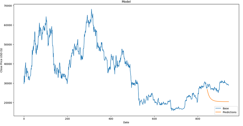

Ouch…

Github link : https://github.com/leopoldcosson/medium