Learning Attention Mechanism from scratch!

because Attention Is All You Need, literally!

“One important property of human perception is that one does not tend to process a whole scene in its entirety at once. Instead, humans focus attention selectively on parts of the visual space to acquire information when and where it is needed and combine information from different fixations over time to build up an internal representation of the scene, guiding future eye movements and decision making” — Recurrent Models of Visual Attention,2014

In this post, I will show you how attention is implemented. The main focus would be on implementing attention in isolation from a larger model. That’s because when we implement attention in a real-world model, a lot of the focus goes into piping the data and juggling numerous vectors rather than the concepts of attention themselves.

I will implement attention scoring as well as calculating an attention context vector.

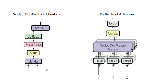
Attention Scoring:

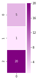
Let’s start by looking at the inputs we’ll give to the scoring function. We will assume we’re in the first step in the decoding phase. The first input to the scoring function is the hidden state of the decoder (assuming a toy RNN with three hidden nodes — not usable in real life, but easier to illustrate)

dec_hidden_state = [5,1,20]

Let’s visualize this vector:

%matplotlib inline
import numpy as np
import matplotlib.pyplot as plt
import seaborn as sns

Let’s visualize our decoder hidden state:

plt.figure(figsize=(1.5, 4.5))
sns.heatmap(np.transpose(np.matrix(dec_hidden_state)), annot=True, cmap=sns.light_palette(“purple”, as_cmap=True), linewidths=1)

You’ll get something like this:

Our first scoring function will score a single annotation (encoder hidden state), which looks like this:

annotation = [3,12,45] #e.g. Encoder hidden state

Let’s visualize the single annotation:

plt.figure(figsize=(1.5, 4.5))
sns.heatmap(np.transpose(np.matrix(annotation)), annot=True, cmap=sns.light_palette(“orange”, as_cmap=True), linewidths=1)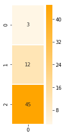

IMPLEMENT: Scoring a Single Annotation

Let’s calculate the dot product of a single annotation.

NumPy’s dot() is a good candidate for this operation

def single_dot_attention_score(dec_hidden_state, enc_hidden_state):
 #return the dot product of the two vectors
 return np.dot(dec_hidden_state, enc_hidden_state)
 
single_dot_attention_score(dec_hidden_state, annotation)

Result: 927

Annotations Matrix

Let’s now look at scoring all the annotations at once. To do that, here’s our annotation matrix:

annotations = np.transpose([[3,12,45], [59,2,5], [1,43,5], [4,3,45.3]])

And it can be visualized like this (each column is a hidden state of an encoder time step):

ax = sns.heatmap(annotations, annot=True, cmap=sns.light_palette(“orange”, as_cmap=True), linewidths=1)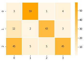

IMPLEMENT: Scoring All Annotations at Once

Let’s calculate the scores of all the annotations in one step using matrix multiplication. Let’s continue to use the dot scoring method but to do that, we’ll have to transpose dec_hidden_state and matrix multiply it with annotations.

def dot_attention_score(dec_hidden_state, annotations):
 # return the product of dec_hidden_state transpose and enc_hidden_states
 return np.matmul(np.transpose(dec_hidden_state), annotations)
 
attention_weights_raw = dot_attention_score(dec_hidden_state, annotations)
attention_weights_raw

Now that we have our scores, let’s apply softmax:

def softmax(x):
 x = np.array(x, dtype=np.float128)
 e_x = np.exp(x)
 return e_x / e_x.sum(axis=0)

attention_weights = softmax(attention_weights_raw)
attention_weights

Applying the scores back on the annotations

Now that we have our scores, let’s multiply each annotation by its score to proceed closer to the attention context vector. This is the multiplication part of this formula (we’ll tackle the summation part in the latter cells)

def apply_attention_scores(attention_weights, annotations):
 # Multiple the annotations by their weights
 return attention_weights * annotations

applied_attention = apply_attention_scores(attention_weights, annotations)
applied_attention

Let’s visualize how the context vector looks now that we’ve applied the attention scores back on it:

# Let’s visualize our annotations after applying attention to them
ax = sns.heatmap(applied_attention, annot=True, cmap=sns.light_palette(“orange”, as_cmap=True), linewidths=1)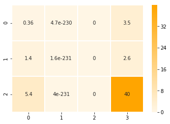

Contrast this with the raw annotations visualized earlier, and we can see that the second and third annotations (columns) have been nearly wiped out. The first annotation maintains some of its value, and the fourth annotation is the most pronounced.

Calculating the Attention Context Vector

All that remains to produce our attention context vector now is to sum up the four columns to produce a single attention context vector

def calculate_attention_vector(applied_attention):
 return np.sum(applied_attention, axis=1)

attention_vector = calculate_attention_vector(applied_attention)
attention_vector

# Let’s visualize the attention context vector
plt.figure(figsize=(1.5, 4.5))
sns.heatmap(np.transpose(np.matrix(attention_vector)), annot=True, cmap=sns.light_palette(“Blue”, as_cmap=True), linewidths=1)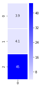

Now that we have the context vector, we can concatenate it with the hidden state and pass it through a hidden layer to provide the result of this decoding time step.

So, in this blog post, we learned all about attention scoring, scoring a single & all annotations, annotation matrix, applying the scores back on the annotations. I hope, isolating attention implementation from a larger model made concepts of attention a bit more clear.

If you want to check the code out all at once, please refer: Attention Basics