
Learn to Calculate Your Portfolio’s Value at Risk
Step by Step Guide to Risk Managing Your Portfolio with Historical VaR and Expected Shortfall
In this article, we are going to learn about risk management and how we can apply it to our equity portfolios. We are going to do that by learning about two risk management metrics, Value at Risk (VaR) and Expected Shortfall (ES) while also going through a step by step guide on how you can build a model to calculate these metrics specifically for your portfolio.

What is VaR?
The best way to explain VaR is to pose the question it helps answer:
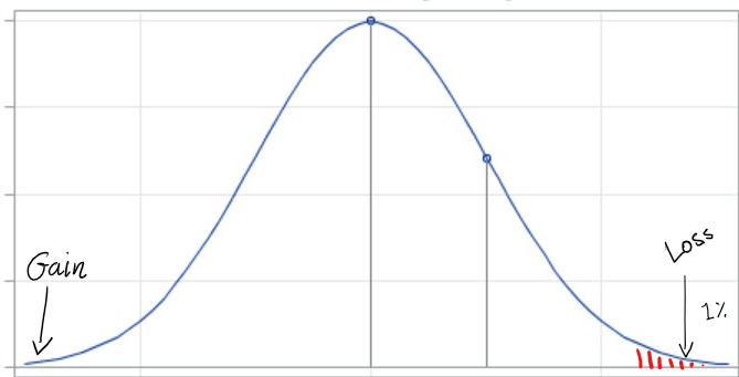
What is the maximum loss I can expect my portfolio to have with a time horizon X and a certainty of Y%?
In other words, a one day 99% VaR of $100, means that my portfolio’s one-day maximum loss for 99% of the times, would be less than $100.
We can essentially calculate VaR from the probability distribution of the portfolio losses.
How do you calculate VaR?
There are several different methodologies that one can use to calculate VaR. The three most common ones are:
- Historical Simulation
- Monte Carlo
- Variance Covariance
In this blog, we will only cover Historical Simulation.
What is VaR Historical Simulation?
The Historical Simulation Method entails calculating daily portfolio changes in value to determine the probability distribution of returns. It does that by looking at how your portfolio would have behaved historically.
Once you have your portfolio’s returns or losses, you can calculate within a confidence interval the worst possible outcome.
What are the mechanics of calculating VaR using Historical Simulation?
- Using historical data, determine your portfolio’s value for a number of days (typically around 500)
- Calculate the % change between each day
- Using your current portfolio valuation, calculate the monetary impact of the % change.
- Sort your results from the highest loss to most profit
- Depending on your confidence interval, the nth value that corresponds to that percentage — This is your one day VaR.
- Multiply it by the square root of the number of days you want your time horizon to be, i.e. 5day VaR = 1day VaR * sqr(5) (This is because the returns are assumed to be independently and identically distributed (normal with mean 0)) (Note: I will show you how we can check this at the end of our implementation)
What are the limitations of VaR?
As with any metric, there are advantages and disadvantages. VaR is so widely used because it’s straightforward to understand. However, it does come with some drawbacks:
- VaR assumes slim tails, i.e. Tail risk is not sufficiently captured.
- VaR doesn’t consider black swan events, i.e. things that happen rarely and unexpectedly (unless within your look-up set)
- Historical VaR is slow to capturing changing market conditions as it assumes past performance represents future performance.
What is Expected Shortfall (ES)?
Expected Shortfall, is a risk metric that attempts to address one of the drawbacks of VaR. VaR assumes that the risk in the tail-end of the distribution is improbable with a thin tail. However, not surprisingly, in the real world we have seen distributions where the tail is quite fat:

To address that, ES takes the average of the tail.
Calculating the Historical VaR and ES for our portfolio in Python
First up, we need to define our portfolio holdings.
import pandas as pddata = {'Stocks':['GOOGL', 'TSLA','AAPL'], 'Quantity':[100, 50, 300]} #Define your holdings# Create a DataFrame of holdings
df = pd.DataFrame(data)With our holdings defined, we need to source historic prices for each of our stocks that will allow us to value our portfolio (if you need to see different options and sourcing for sourcing historical data, check out my previous blog). In this instance, I am using the Tiingo API, which will result in a pandas dataframe:
from tiingo import TiingoClientdef SourceHistoricPrices():
if info == 1: print('[INFO] Fetching stock prices for portfolio holdings')
#Set Up for Tiingo
config = {}
config['session'] = True
config['api_key'] = 'private key'
client = TiingoClient(config)
#Create a list of tickers for the API call
Tickers = []
i=0
for ticker in data:
while i <= len(data):
Tickers.append(data[ticker][i])
i=i+1
if info == 1: print('[INFO] Portfolio Holdings determined as', Tickers)
if info == 1: print('[INFO] Portfolio Weights determined as', data['Quantity'])
#Call the API and store the data
global HistData
HistData = client.get_dataframe(Tickers, metric_name='close', startDate=dateforNoOfScenarios(today), endDate=today)
if info == 1: print('[INFO] Fetching stock prices completed.', len(HistData), 'days.')
return(HistData)One thing to note here is that we need to define the start and end date by which we require historical data which will drive the number of historical simulations. This should be a user-defined input. A slight problem with that, however, is that the stock market is not open every day. Hence, we need to calculate the business days involved. Without include, a holiday calendar is quite hard to be precise, but for our purposes, a quick approximation should suffice.
ScenariosNo = 500 #Define the number of scenarios you want to runtoday = datetime.date.today() - datetime.timedelta(days=1)def is_business_day(date):
return bool(len(pd.bdate_range(date, date)))def dateforNoOfScenarios(date):
i=0
w=0
while i < ScenariosNo:
if (is_business_day(today - datetime.timedelta(days = w)) == True):
i = i+1
w = w+1
else:
w = w+1
continue
#print('gotta go back these many business days',i)
#print('gotta go back these many days',w)
#remember to add an extra day as percentage difference will leave first value blank (days +1 = scenario numbers)
return(today - datetime.timedelta(days = w*1.04 + 1)) #4% is an arbitrary number I've calculated the holidays to be in 500days.Next up, we need to value our portfolio.
def ValuePortfolio():
    HistData['PortValue'] = 0
    i=0
    if info == 1: print('[INFO] Calculating the portfolio value for each day')
    while i<= len(data):
        stock = data['Stocks'][i]
        quantity = data['Quantity'][i]
        HistData['PortValue'] = HistData[stock] * quantity + HistData['PortValue']
        i = i+1
which results in:
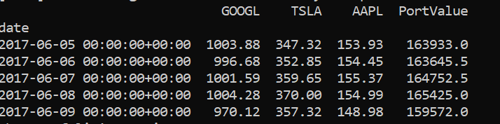
So now, we can go ahead and calculate the percentage change:
def CalculateVaR():
    if info == 1: print('[INFO] Calculating Daily % Changes')
    HistData['Perc_Change'] = HistData['PortValue'].pct_change() #calculating percentage change
Then the portfolio’s valuation change:
HistData['DollarChange'] = HistData.loc[HistData.index.max()]['PortValue'] * HistData['Perc_Change'] #calculate money change based on current valuation
if info == 1: print('[INFO] Picking', round(HistData.loc[HistData.index.max()]['PortValue'],2),' value from ', HistData.index.max().strftime('%Y-%m-%d'), ' as the latest valuation to base the monetary returns')
Then determine the n-th value we need to pick for our confidence interval:
ValueLocForPercentile = round(len(HistData) * (1 - (Percentile / 100)))
if info == 1: print('[INFO] Picking the', ValueLocForPercentile, 'th highest value')
Sort the data and select the value:
global SortedHistData
SortedHistData = HistData.sort_values(by=['DollarChange'])
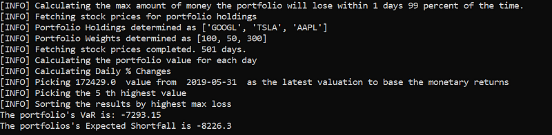
if info == 1: print('[INFO] Sorting the results by highest max loss')and finally, calculate our portfolio’s VaR value:
VaR_Result = SortedHistData.iloc[ValueLocForPercentile + 1,len(SortedHistData.columns)-1] * np.sqrt(VarDaysHorizon)print('The portfolio\'s VaR is:', round(VaR_Result,2))Resulting in:
Putting it all together gives:
from tiingo import TiingoClient
import pandas as pd, datetime, numpy as np
import matplotlib.pyplot as plt
import warnings
warnings.filterwarnings('ignore') #Tiingo API is returning a warning due to an upcoming pandas update#User Set Up
data = {'Stocks':['GOOGL', 'TSLA','AAPL'], 'Quantity':[100, 50, 300]} #Define your holdings
ScenariosNo = 500 #Define the number of scenarios you want to run
Percentile = 99 #Define your confidence interval
VarDaysHorizon = 1 #Define your time period
info = 1 #1 if you want more info returned by the script# Create a DataFrame of holdings
df = pd.DataFrame(data)
print('[INFO] Calculating the max amount of money the portfolio will lose within', VarDaysHorizon, 'days', Percentile, 'percent of the time.')today = datetime.date.today() - datetime.timedelta(days=1)def is_business_day(date):
return bool(len(pd.bdate_range(date, date)))def dateforNoOfScenarios(date):
i=0
w=0
while i < ScenariosNo:
if (is_business_day(today - datetime.timedelta(days = w)) == True):
i = i+1
w = w+1
else:
w = w+1
continue
#print('gotta go back these many business days',i)
#print('gotta go back these many days',w)
#remember to add an extra day (days +1 = scenario numbers)
return(today - datetime.timedelta(days = w*1.04 + 1)) #4% is an arbitary number i've calculated the holidays to be in 500days.def SourceHistoricPrices():
if info == 1: print('[INFO] Fetching stock prices for portfolio holdings')
#Set Up for Tiingo
config = {}
config['session'] = True
config['api_key'] = 'private key'
client = TiingoClient(config)
#Create a list of tickers for the API call
Tickers = []
i=0
for ticker in data:
while i <= len(data):
Tickers.append(data[ticker][i])
i=i+1
if info == 1: print('[INFO] Portfolio Holdings determined as', Tickers)
if info == 1: print('[INFO] Portfolio Weights determined as', data['Quantity'])
#Call the API and store the data
global HistData
HistData = client.get_dataframe(Tickers, metric_name='close', startDate=dateforNoOfScenarios(today), endDate=today)
if info == 1: print('[INFO] Fetching stock prices completed.', len(HistData), 'days.')
return(HistData)def ValuePortfolio():
HistData['PortValue'] = 0
i=0
if info == 1: print('[INFO] Calculating the portfolio value for each day')
while i<= len(data):
stock = data['Stocks'][i]
quantity = data['Quantity'][i]
HistData['PortValue'] = HistData[stock] * quantity + HistData['PortValue']
i = i+1def CalculateVaR():
if info == 1: print('[INFO] Calculating Daily % Changes')
#calculating percentage change
HistData['Perc_Change'] = HistData['PortValue'].pct_change()
#calculate money change based on current valuation
HistData['DollarChange'] = HistData.loc[HistData.index.max()]['PortValue'] * HistData['Perc_Change']
if info == 1: print('[INFO] Picking', round(HistData.loc[HistData.index.max()]['PortValue'],2),' value from ', HistData.index.max().strftime('%Y-%m-%d'), ' as the latest valuation to base the monetary returns')
ValueLocForPercentile = round(len(HistData) * (1 - (Percentile / 100)))
if info == 1: print('[INFO] Picking the', ValueLocForPercentile, 'th highest value')
global SortedHistData
SortedHistData = HistData.sort_values(by=['DollarChange'])
if info == 1: print('[INFO] Sorting the results by highest max loss')
VaR_Result = SortedHistData.iloc[ValueLocForPercentile + 1,len(SortedHistData.columns)-1] * np.sqrt(VarDaysHorizon)
print('The portfolio\'s VaR is:', round(VaR_Result,2))def CalculateES():
ValueLocForPercentile = round(len(HistData) * (1 - (Percentile / 100)))
ES_Result = round(SortedHistData['DollarChange'].head(ValueLocForPercentile).mean(axis=0),2) * np.sqrt(VarDaysHorizon)
print('The portfolios\'s Expected Shortfall is', ES_Result)SourceHistoricPrices()
ValuePortfolio()
CalculateVaR()
CalculateES()Finally, we can also use a histogram to see how our portfolio returns fit with the assumption that we’ve made in point 6 above:
The reason we can extend 1 day VaR or ES by multiplying by the Square Root of days, it is because the returns are assumed to be independently and identically distributed (normal with mean 0)
import scipy
import scipy.stats, matplotlib.pyplot as plt
def plotme():
data1 = HistData['Perc_Change']
num_bins = 50
# the histogram of the data
n, bins, patches = plt.hist(data1, num_bins, normed=1, facecolor='green', alpha=0.5)
# add a 'best fit' line
sigma = HistData['Perc_Change'].std()
data2 = scipy.stats.norm.pdf(bins, 0, sigma)
plt.plot(bins, data2, 'r--')
plt.xlabel('Percentage Change')
plt.ylabel('Probability/Frequency')
# Tweak spacing to prevent clipping of ylabel
plt.subplots_adjust(left=0.15)
plt.show()plotme()Returning:
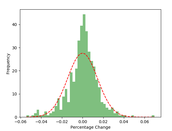
We are hence validating our assumption.
If you liked this blog post, you might also like: