Lasso Regression: A Comprehensive Guide to Feature Selection and Regularization

In the world of machine learning and statistical modeling, Lasso regression (short for “Least Absolute Shrinkage and Selection Operator”) is a widely employed technique that provides valuable insights into feature selection and regularization. This blog post aims to serve as a comprehensive guide to understanding Lasso regression, covering its fundamental concepts, mathematical formulation, and implementation in Python.

Understanding Linear Regression

Linear regression is a fundamental technique in statistical modeling used to establish a linear relationship between a dependent variable and one or more independent variables. It serves as the foundation for more advanced regression techniques like Lasso regression.

Basic Equation: The basic equation of linear regression can be represented as follows:

y = β₀ + β₁x₁ + β₂x₂ + … + βₚxₚ + ɛ

where:

y is the dependent variable (also known as the target or response variable).
β₀ represents the intercept term.
β₁, β₂, ..., βₚ are the regression coefficients associated with the independent variables x₁, x₂, ..., xₚ.
ɛ is the error term, which captures the unexplained variability or noise in the relationship between the dependent and independent variables.

The goal of linear regression is to estimate the regression coefficients (β₀, β₁, β₂, ..., βₚ) that best fit the observed data, minimizing the sum of squared residuals between the predicted and actual values.

Assumptions: Linear regression relies on certain assumptions to provide reliable estimates of the regression coefficients and accurate predictions. These assumptions include:

Linearity: The relationship between the dependent variable and the independent variables is assumed to be linear.
Independence: The observations are assumed to be independent of each other.
Homoscedasticity: The variance of the error term is constant across all levels of the independent variables.
Normality: The error term is assumed to follow a normal distribution.

Introducing Lasso Regression

Lasso regression, short for “Least Absolute Shrinkage and Selection Operator,” is an extension of linear regression that combines both feature selection and regularization. It achieves this by introducing a penalty term based on the L1 norm of the regression coefficients. Let’s look into the mathematical equation of Lasso regression to understand these concepts.

Objective Function:

The objective function of Lasso regression is formulated as a combination of the least squares term and the L1 norm penalty term. It aims to minimize the sum of squared residuals between the predicted and actual values, while simultaneously adding a penalty on the magnitude of the regression coefficients.

The mathematical equation for Lasso regression can be represented as follows:

minimize 1/(2n) * Σ(yᵢ — (β₀ + ΣβⱼXⱼᵢ))² + α * Σ|βⱼ|

where:

n represents the number of samples in the dataset.
yᵢ denotes the observed value of the dependent variable for the i-th sample.
Xⱼᵢ represents the value of the j-th predictor (feature) for the i-th sample.
β₀ is the intercept term.
βⱼ represents the regression coefficient associated with the j-th predictor.

The first part of the objective function, 1/(2n) * Σ(yᵢ - (β₀ + ΣβⱼXⱼᵢ))², is the least squares term. It measures the squared difference between the observed values and the predicted values based on the regression equation.

The second part of the objective function, α * Σ|βⱼ|, is the L1 norm penalty term. It encourages sparsity in the model by promoting some of the regression coefficients to become exactly zero. The tuning parameter α controls the strength of the penalty, with larger values of α leading to more coefficients being driven to zero.

Feature Selection and Regularization:

Lasso regression’s ability to perform feature selection stems from the L1 norm penalty term. By driving some regression coefficients to zero, Lasso regression identifies and prioritizes the most relevant features. This promotes sparsity in the model and enables automatic feature selection, which is particularly useful when dealing with high-dimensional datasets.

Additionally, Lasso regression provides regularization by controlling the complexity of the model. The penalty term helps prevent overfitting by shrinking the coefficients and discouraging excessive complexity. Regularization improves the model’s generalization ability, allowing it to perform well on unseen data.

By combining feature selection and regularization, Lasso regression strikes a balance between simplicity and predictive power, making it a valuable tool in various domains.

Key Concepts of Lasso Regression

In this section, we’ll explore two key concepts of Lasso regression: the L1 norm penalty and the tuning parameter alpha. Understanding these concepts is essential to grasp the underlying principles and advantages of Lasso regression.

L1 Norm Penalty: The L1 norm penalty is a crucial component of Lasso regression that promotes sparsity and facilitates feature selection. It is based on the sum of the absolute values of the regression coefficients.

The L1 norm penalty term in the objective function of Lasso regression, α * Σ|βⱼ|, encourages some coefficients to become exactly zero. This leads to a sparse model where only a subset of features have non-zero coefficients, effectively performing feature selection. The remaining features with zero coefficients are deemed less relevant to the target variable.

The L1 norm penalty helps identify and prioritize the most influential predictors, making the model more interpretable and reducing the impact of irrelevant or redundant features. This feature selection capability is particularly valuable when working with datasets that contain a large number of features.

Tuning Parameter: Alpha: The tuning parameter alpha (α) plays a crucial role in controlling the trade-off between model complexity and the degree of sparsity in Lasso regression. It determines the strength of the L1 norm penalty and influences the behavior of the regression coefficients.

By adjusting the value of alpha, we can control the amount of regularization applied in Lasso regression. Larger values of alpha result in stronger regularization, pushing more coefficients towards zero and promoting sparser models. Smaller values of alpha, on the other hand, lead to less regularization, allowing for a greater number of non-zero coefficients.

The selection of an appropriate alpha value depends on the specific dataset and the desired level of sparsity. It is often determined using techniques such as cross-validation or information criteria, where different alpha values are tested, and the one that yields the best model performance is selected.

Choosing the optimal alpha value is crucial to achieve the desired level of feature selection and regularization in Lasso regression. It requires careful consideration and understanding of the dataset and the problem at hand.

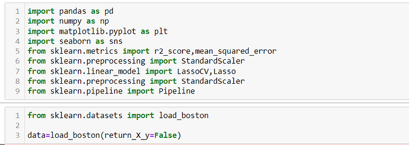
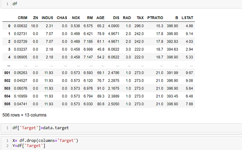
Lets use the load_boston function from scikit-learn's datasets module to load the Boston Housing dataset. The dataset is stored in the data variable, then create a pandas DataFrame (df) to store the dataset's feature data and assigns column names along with target variable is added to the DataFrame, and the feature matrix (X) and target variable (Y) are separated for further analysis.

Use scikit-learn’s train_test_split function to split the dataset into training and testing sets (X_train, X_test, y_train, y_test) with a 70:30 ratio.

Let’s start by applying linear regression to the Boston Housing dataset. We will calculate the R-squared score and mean squared error to evaluate the performance of the model.

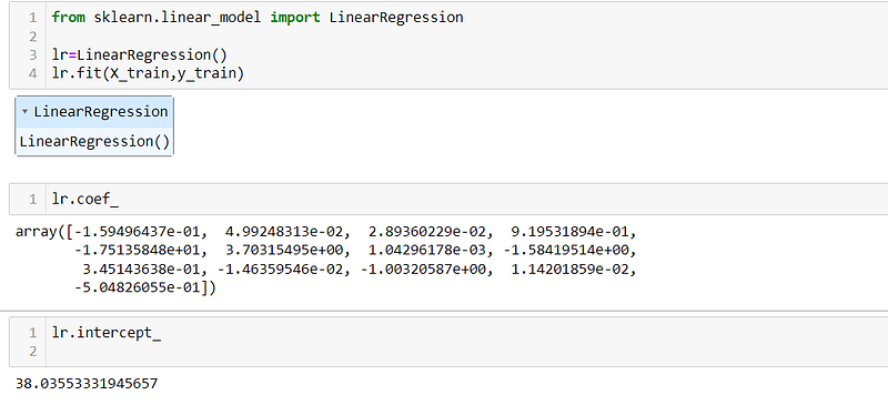
By applying linear regression to the Boston Housing dataset, we can observe the coefficients and intercept of the model. These values represent the parameters of the best-fit line that the linear regression model has learned, allowing us to understand the relationship between the input features and the target variable in the dataset.

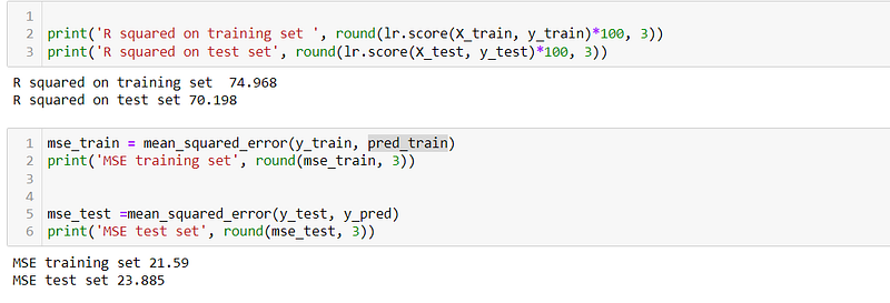
The R2 score for training and testing data is 74.968 and 70198 and Mean Squared Error is 21.59 and 23.885 respectively.

Now let’s analyze using Lasso regression from the scikit-learn library. We will set the alpha parameter to 1, which controls the strength of regularization in Lasso regression. By applying Lasso regression with this alpha value, we can evaluate its impact on feature selection and regularization.

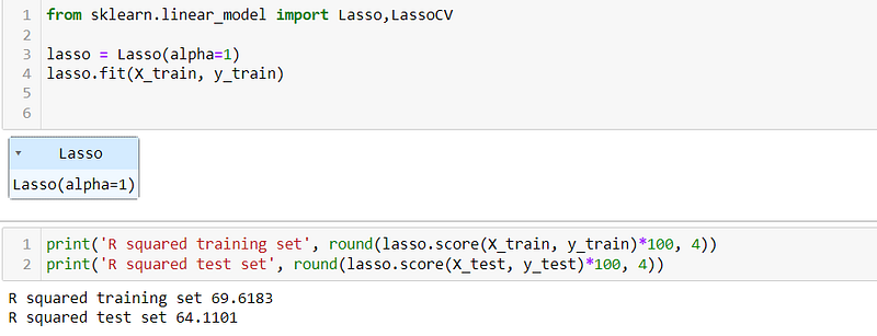
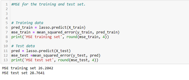
We can see the R2 score for training dataset is 69.61, and testing data is 64.1101, similarly the MSE for training and testing data is 26.2042 and 28.7641

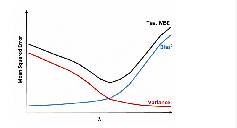
The reduced R-squared score and increased mean squared error (MSE) for the testing data compared to the training data in Lasso regression can be attributed to the effect of regularization.

When the R-squared score decreases and the MSE increases for the testing data compared to the training data, it indicates that the model’s performance is slightly worse on unseen data. This difference can be attributed to the regularization applied by Lasso regression.

To gain a better understanding of the impact of the alpha parameter in Lasso regression, we plot the coefficients of the Lasso model as a function of alpha. The plot allows us to visualize how the coefficients change with varying alpha values. The max_iter parameter determines the maximum number of iterations allowed for the Lasso algorithm to converge.

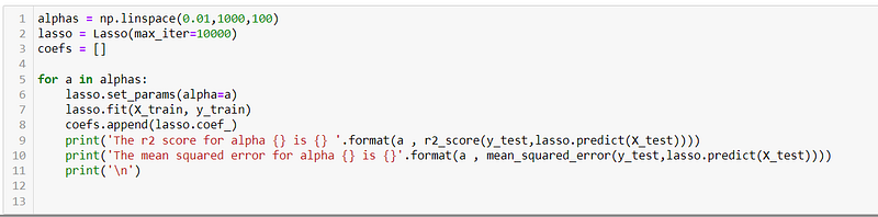
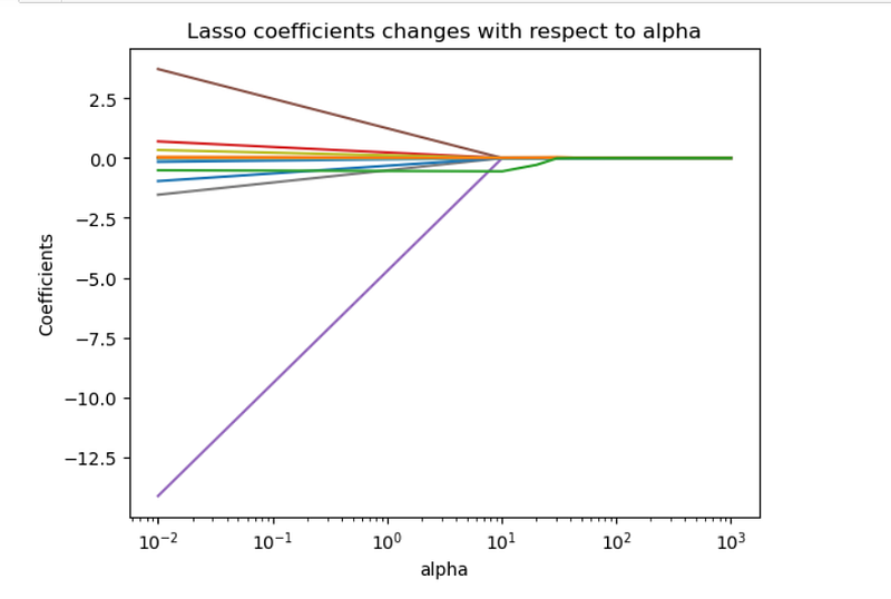
In the plotted graph, as we move from left to right, we can observe the effect of increasing alpha values on the Lasso models.

When alpha is set to 0, the Lasso regression behaves similarly to the least squares fit, where all predictor variables are considered, and the coefficient estimates are not constrained to be zero.

As we increase the alpha value, the Lasso regression gradually introduces more sparsity into the model. This means that some predictor variables start to have their coefficient estimates shrink towards zero. Features that are less relevant or have weaker associations with the target variable are more likely to have their coefficients approach zero faster as alpha increases.

At very large alpha values, the Lasso regression tends towards the null model, where all coefficient estimates are forced to be exactly zero. In this scenario, the model becomes extremely sparse, selecting only a subset of the most important predictors that have the strongest impact on the target variable.

Lasso with Optimal Alpha

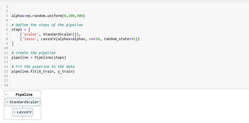
To determine the optimal value of alpha for Lasso regression, we can utilize scikit-learn’s LassoCV (Lasso Cross-Validation) module. This approach involves iterative fitting along a regularization path and selecting the best model based on cross-validation.

K-fold Cross-Validation

To find the best alpha value, we employ k-fold cross-validation. This technique involves dividing the dataset into k equally-sized folds, where each fold serves as both a training and validation set. The LassoCV algorithm fits the Lasso model multiple times, each time using a different alpha value and evaluating the model’s performance on the validation set.

By leveraging k-fold cross-validation, we can assess how well the Lasso model generalizes to unseen data. The optimal alpha value is determined by selecting the alpha that yields the best model performance across all the folds, typically measured by metrics such as mean squared error or R-squared score.

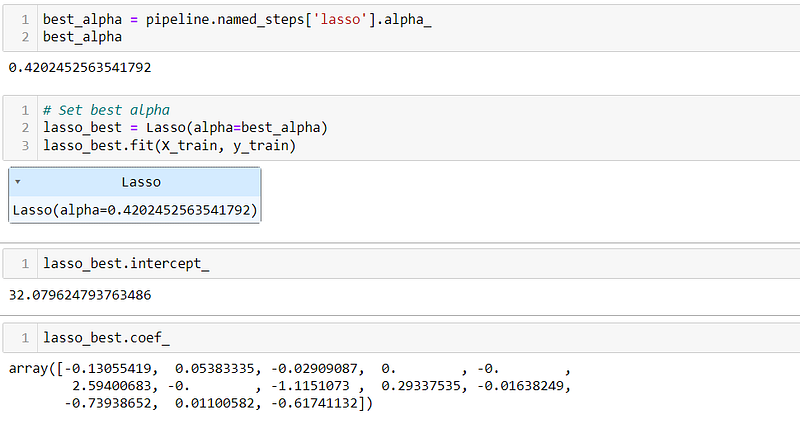
Lets fit the data using the best alpha calculated above using lasso.

Linear Regression:

Coefficients: The Linear Regression model has non-zero coefficients for all the features. Each coefficient represents the impact of the corresponding feature on the target variable. For example, a positive coefficient indicates a positive relationship, while a negative coefficient indicates a negative relationship.
Intercept: The intercept term in Linear Regression is 38.0355, which represents the predicted value of the target variable when all predictor variables are zero. It is an additive constant that adjusts the regression line.
R-squared: The R-squared score measures the proportion of variance in the target variable that is explained by the model. The Linear Regression model achieves an R-squared score of 74.968% on the training set and 70.198% on the test set. This indicates that the model explains approximately 74.968% of the variance in the training set and 70.198% of the variance in the test set.
Mean Squared Error (MSE): The MSE quantifies the average squared difference between the predicted and actual values. The Linear Regression model yields an MSE of 21.59 on the training set and 23.885 on the test set. A lower MSE indicates better prediction accuracy.

Lasso Regression with best alpha:

Coefficients: The Lasso Regression model introduces sparsity by assigning zero coefficients to certain features. This feature selection property of Lasso helps identify the most relevant predictors. The coefficients in the Lasso model represent the impact of the corresponding features on the target variable. For example, a non-zero coefficient indicates the feature’s importance, while a zero coefficient suggests the feature’s exclusion from the model.
Intercept: The intercept term in Lasso Regression is 32.0796, similar to Linear Regression. It represents the predicted value of the target variable when all predictor variables are zero.
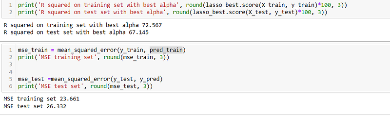
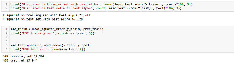
R-squared: The Lasso Regression model achieves an R-squared score of 73.093% on the training set and 67.629% on the test set when using the best alpha value. This indicates that the Lasso model explains approximately 73.093% of the variance in the training set and 67.629% of the variance in the test set.
Mean Squared Error (MSE): The Lasso Regression model yields an MSE of 23.208 on the training set and 25.944 on the test set. The slightly higher MSE compared to Linear Regression suggests that the Lasso model’s predictions deviate slightly more from the actual values.

Comparison:

Linear Regression: The model includes all the features with non-zero coefficients, providing a complete view of the predictors’ impact on the target variable. The R-squared scores indicate a good level of explained variance, and the MSE values are relatively low.
Lasso Regression: The model performs feature selection by assigning zero coefficients to some features, identifying the most important predictors. This leads to a more interpretable and potentially simpler model. The R-squared scores and MSE values, although slightly lower compared to Linear Regression, still indicate a reasonable level of prediction accuracy.

Conclusion:

Lasso regression is a valuable technique for feature selection and regularization in linear regression models. By penalizing the sum of absolute coefficients, it effectively shrinks less important features to zero, improving model interpretability and reducing overfitting. In this blog post, we discussed the concepts of lasso regression, provided a practical implementation in Python using scikit-learn, and visualized the effect of different alpha values on the coefficients.