
Kalman Filters for Stock Price Signal Generation
Let’s implement a Kalman filter for predicting stock prices using synthetic data.
Overview:
- Generate synthetic stock price data.
- Implement a Kalman filter for the synthetic stock data.
- Demonstrate how the Kalman filter can be used to dynamically adjust predictions and trading strategies.
Step 1: Generate Synthetic Stock Price Data
To begin, we’ll generate synthetic stock price data. We’ll use a simple random walk model with some noise:
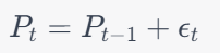
Where Pt is the stock price at time t, and ϵt is a random noise term.
import numpy as np
import matplotlib.pyplot as plt

# Seed for reproducibility
np.random.seed(42)

# Number of days for our synthetic stock data
num_days = 250

# Generate synthetic stock price data using random walk
epsilon = np.random.normal(0, 2, num_days)  # Noise term
prices = np.cumsum(epsilon) + 50  # Start from a stock price of 50

# Plot the synthetic stock price data
plt.figure(figsize=(10, 6))
plt.plot(prices, label="Synthetic Stock Price")
plt.title("Synthetic Stock Price Data")
plt.xlabel("Days")
plt.ylabel("Stock Price")
plt.legend()
plt.grid(True)
plt.show()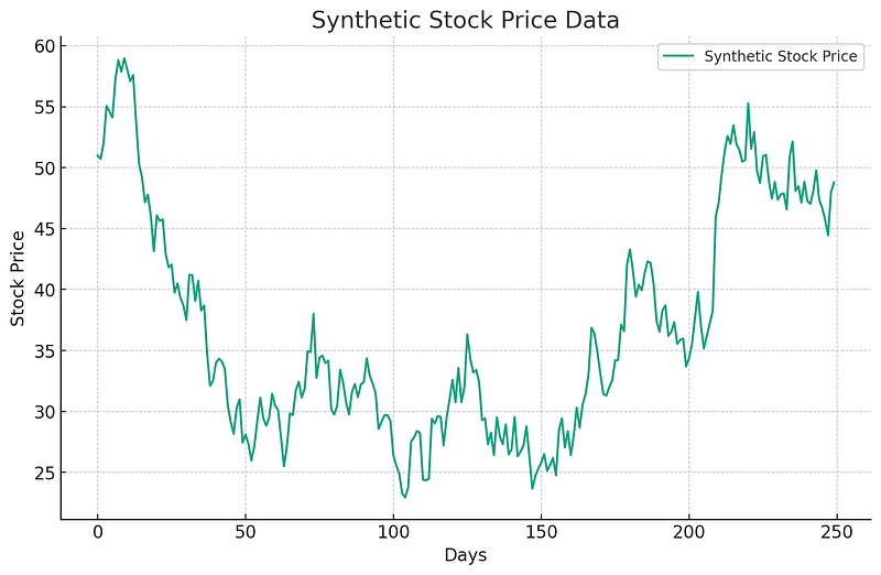
Here’s our synthetic stock price data based on the random walk model. The stock price starts at 50 and evolves over 250 days.
Step 2: Implement a Kalman Filter for the Synthetic Stock Data
The Kalman filter is a recursive algorithm used to estimate the state of a linear dynamic system from noisy observations. For our stock price prediction, we’ll use the following simple model:
State equation:
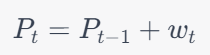
Where Pt is the true stock price at time t, and wt is the process noise which is assumed to be normally distributed with mean 0 and variance Q.
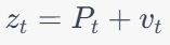
Observation equation:
Let’s implement the Kalman filter for our synthetic stock price data:
class KalmanFilter:
    def __init__(self, Q, R):
        # Initial state estimate
        self.P_hat = np.zeros(num_days)
        # Initial state estimate error variance
        self.P_var = np.zeros(num_days)
        # Process noise variance
        self.Q = Q
        # Measurement noise variance
        self.R = R
        # Initial estimate of state
        self.P_hat[0] = prices[0]
        # Initial estimate of state variance
        self.P_var[0] = 1.0

    def update(self, z):
        for t in range(1, num_days):
            # Prediction Step
            P_hat_minus = self.P_hat[t-1]  # Predicted state estimate
            P_var_minus = self.P_var[t-1] + self.Q  # Predicted error variance

            # Update Step
            Kt = P_var_minus / (P_var_minus + self.R)  # Kalman gain
            self.P_hat[t] = P_hat_minus + Kt * (z[t] - P_hat_minus)  # Updated state estimate
            self.P_var[t] = (1 - Kt) * P_var_minus  # Updated estimate of state variance

# Parameters for our Kalman filter
Q = 1  # Process noise variance (assumption)
R = 4  # Measurement noise variance (based on our synthetic data generation)

# Create and run the Kalman filter
kf = KalmanFilter(Q, R)
kf.update(prices)

# Plot the results
plt.figure(figsize=(10, 6))
plt.plot(prices, label="Synthetic Stock Price", alpha=0.5)
plt.plot(kf.P_hat, label="Kalman Filter Estimate", linestyle="--", color="red")
plt.title("Kalman Filter Estimation of Stock Price")
plt.xlabel("Days")
plt.ylabel("Stock Price")
plt.legend()
plt.grid(True)
plt.show()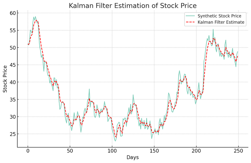
The plot above shows both the synthetic stock price data (in blue) and the Kalman filter estimate (in dashed red). The Kalman filter provides a smoothed estimate of the stock price, reducing the effects of noise.
Step 3: Demonstrate how the Kalman filter can be used to dynamically adjust predictions and trading strategies.
To demonstrate a basic trading strategy, let’s assume the following:
- We buy the stock when the Kalman filter estimate is significantly below the observed price, expecting a price correction upwards.
- We sell the stock when the Kalman filter estimate is significantly above the observed price, expecting a price correction downwards.
For simplicity, we can consider a threshold (e.g., 2 units) to determine when to buy or sell.
Let’s visualize these buy and sell signals on our plot.
# Threshold for buy/sell signals
threshold = 2

# Generate buy/sell signals
buy_signals = np.where(prices < kf.P_hat - threshold)[0]
sell_signals = np.where(prices > kf.P_hat + threshold)[0]

# Plot the results with buy/sell signals
plt.figure(figsize=(12, 7))
plt.plot(prices, label="Synthetic Stock Price", alpha=0.5)
plt.plot(kf.P_hat, label="Kalman Filter Estimate", linestyle="--", color="red")
plt.scatter(buy_signals, prices[buy_signals], marker="^", color="green", s=100, label="Buy Signal")
plt.scatter(sell_signals, prices[sell_signals], marker="v", color="red", s=100, label="Sell Signal")
plt.title("Kalman Filter Estimation with Buy/Sell Signals")
plt.xlabel("Days")
plt.ylabel("Stock Price")
plt.legend()
plt.grid(True)
plt.show()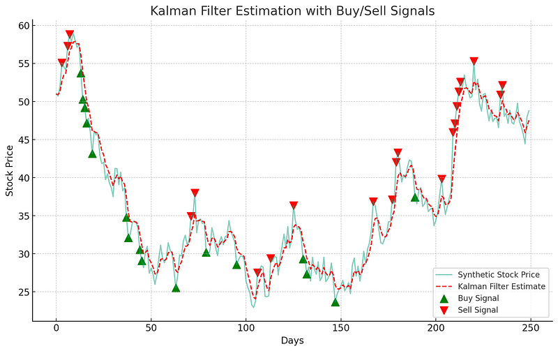
The plot now shows buy signals (green upward triangles) and sell signals (red downward triangles) based on our simple trading strategy using the Kalman filter estimate.
- When the observed stock price is significantly below the Kalman filter estimate (more than our threshold), a buy signal is generated, indicating a potential opportunity to buy the stock in anticipation of a price rise.
- Conversely, when the observed stock price is significantly above the Kalman filter estimate, a sell signal is generated, indicating a potential opportunity to sell the stock in anticipation of a price drop.
Remember, this is a basic demonstration using synthetic data. In a real-world scenario, stock price movements are influenced by many factors, and any trading strategy should be approached with caution and thorough backtesting.


