K-Nearest Neighbor Deconstructed

Application of Nearest Neighbor Search

As beginning Python developers and data scientists, we are introduced to the bevy of libraries that support our work like Numpy, SciPy, Pandas, and SciKit-Learn. These libraries and their packages allow us to fast-track our learning and workflow in parallel. They remove barriers to entry into the technology industry and improve productivity for the beginner and experienced engineer.

However, these out-of-the-box solutions can be challenging to adapt and apply to individual business problems, especially. One issue that only experience can solve is understanding what is happening under the hood when interfacing with a library — what can’t we see on the screen.

An excellent way to gain insight is to build your own algorithm from scratch and then compare it to the library version. This will allow you to deconstruct the algorithm:

● identify what data is and is not in it

● how data structures are manipulated within

● logical sequence

● what mathematical calculations are involved

An additional benefit to building your algorithm is that you have complete control over the code! As your understanding of the algorithm, dataset, data structures, and python itself grows during the exercise (…and, it will), you can adjust the algorithm code itself to reflect your optimization of knowledge and skill.

Build a Classification System Using K-NN

Understanding Classification

Imagine you have a mystery fruit in front of you. You think it could either be a lemon or a lime, but your not too sure. You know limes are small, round, and green, while lemons are usually large, oval-ish, and bright yellow. You haven’t cut your mystery fruit open, so the taste isn’t an observable feature right now.

Let’s just look at color and size to see how K-NN helps us determine what color your mystery fruit is.

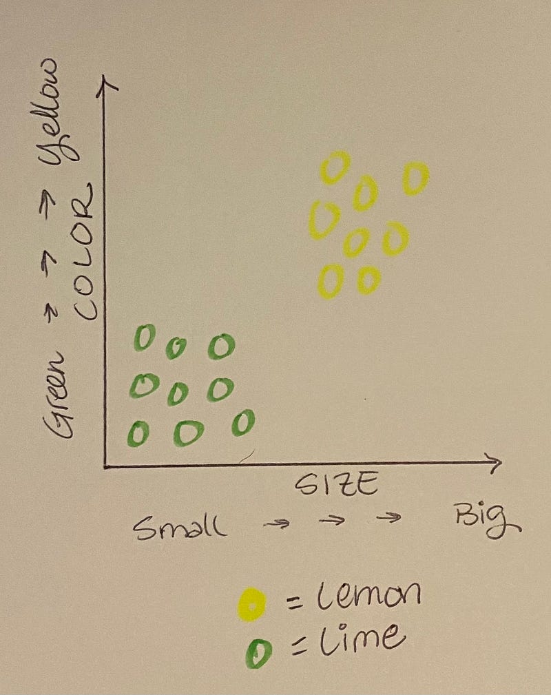
If it’s small and green, the map tells us the fruit is a lime. If it is big and yellow, it is a lemon. What else do we see on the graph? You’re right! All the limes are clustered together, and all the lemons are clustered together.

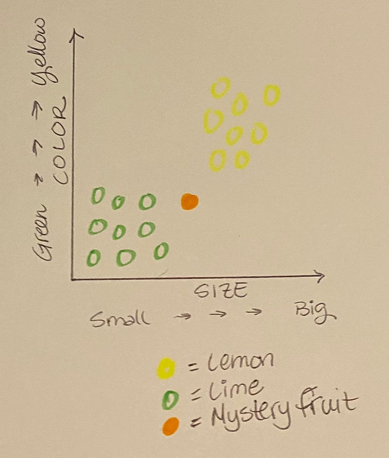
Now we take a look at your mystery fruit. Can you tell by looking at the graph whether it’s a lemon or a lime? Try looking at its nearest neighbors, the closest fruits in straight line distance from its spot on the chart.

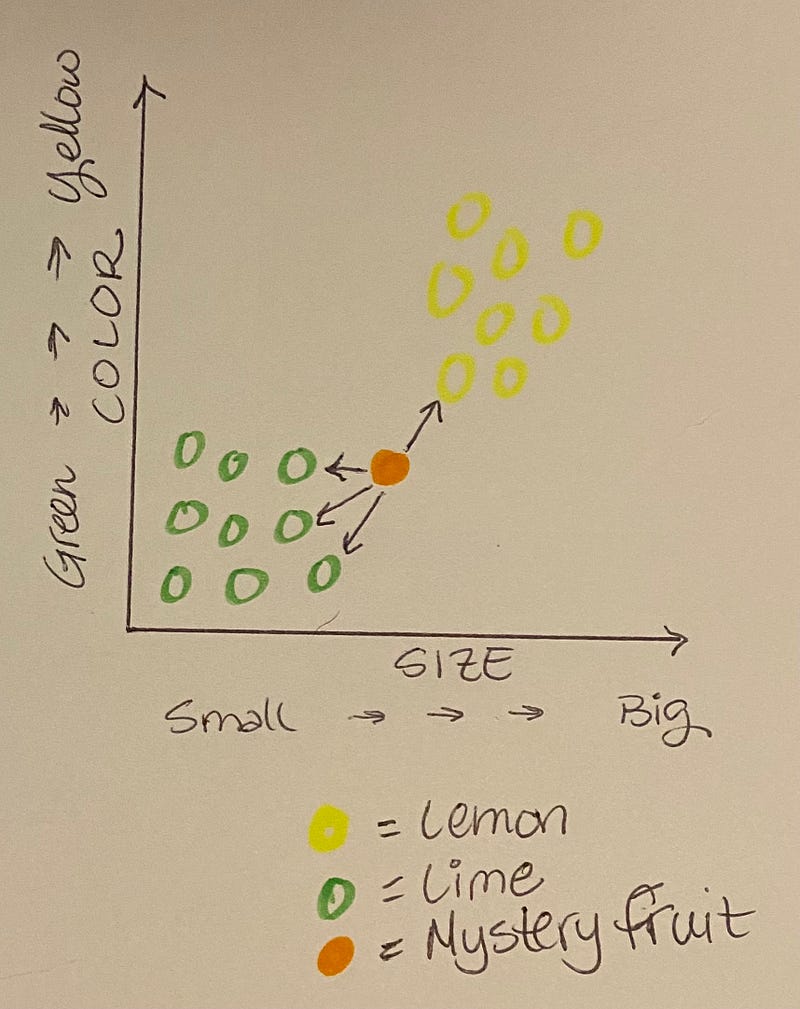
Notice that more of the neighbors are limes than lemons. So, your mystery fruit is probably a lime. Whoo Hoo! you just used the K-Nearest Neighbors to classify your mystery fruit.

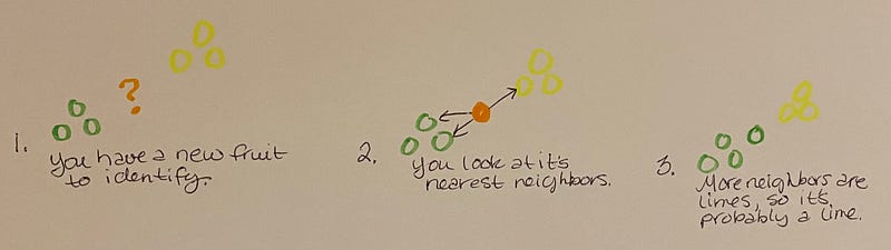
In theory, the algorithm is pretty simple. It is also handy.

Build a K-NN Algorithm from Scratch Using a Python Class

Exploratory Data Analysis

Before we begin, let’s take a quick look at the Iris dataset we use. The Iris dataset contains descriptive information on three species of Irises (the plant). We use this dataset because we can use multiple measurements to solve the taxonomic problem: “Given the measurements of a mystery iris, can we classify it?”

Let’s see if we can identify some relationships or patterns in the measurement data before we begin.

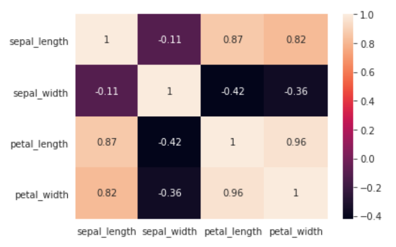
We use the Seaborn library to map the correlations between features. A positive correlation tells us that the two elements have a positive linear relationship. So, as one measurement increases, the other measurement also increases. If a negative correlation exists, there is an inverse relationship where one measurement increases and the other decreases. The closer to 1 or -1 a number is, the stronger the correlation (linear relationship) between the two elements, regardless of whether it’s positive or negative.

We observe the strongest correlations to be (in order of greatest strength):

1. petal_width & petal_length

2. sepal_length & petal_length

3. petal_width & sepal_length

4. sepal_length & petal_width

We note that petal length and width are the most highly correlated with the class. This means that irises in the Iris Virginica class have the longest and widest petals of the three classes of irises in the dataset. Let’s take a look at a broad overview of the inter-correlation of all of these features.

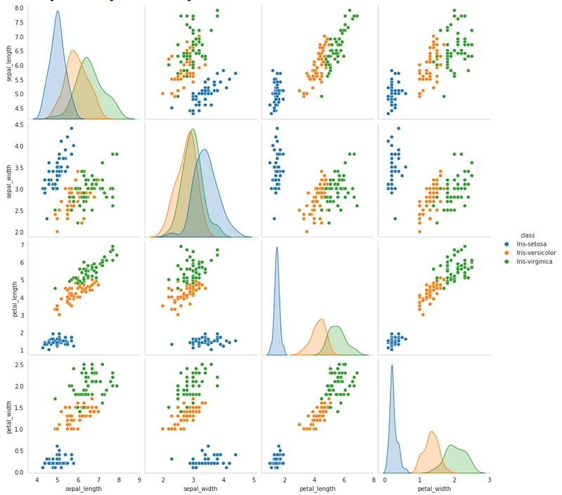
Pair plots allow you to see distributions of individual variables (across the diagonal) and the relationships between two variables within a multi-classification dataset. This is extremely useful in framing our solution to the business problem since we can’t visualize in 4 dimensions or higher.

What we observe in the pair plot:

● a separation of the class Iris Setosa in distribution

● The distinction between classes in petal_length and petal_width

What we infer from the pair plot:

● if 0 <= petal_length <= 2 and 0 <= petal_width <= 0.7, the iris is identified as Iris Setosa

● if 2 <= petal_length <= 5.2 and 1 <= petal_width <= 1.7, the iris is identified as Iris Versicolor

● if None of these is true, the iris is identified as Iris Virginica

Now that we have a good idea of what our data looks like and what it represents, we can begin to develop our model.

Modeling

As we noted in our exploration of the data, the features are strongly linearly correlated yet have differences in distributions among classes. The K-NN algorithm makes predictions by calculating similarities between each instance, in this case, each flower and its measurements, making it the ideal first attempt algorithm to use to solve the mystery flower problem.

Let’s build our algorithm.

To reproduce the From Scratch model, will need to import the following libraries:

● import pandas as pd

● import numpy as np

● import seaborn as sns

Note: The loading of the dataset using the Pandas library is not displayed in this article.

We first build a KNearestNeigbors Python class object (K-NN)that will hold all of our code. Think of it as the ultimate organizer and top level of hierarchy. We load our K-NN instance object using with fields using the __init__ method

class KNearestNeighbors(object):
    def __init__(self, k):
        self.k = k

We create a K-NN instance method to split our dataset into our training dataset and our testing dataset. The benefit of using the Python class structure is that the instance method behaves just like a function and has access to class and instance scope through self.

def train_test_split(dataset, test_size=0.33):
    n_test = int(len(dataset) * test_size)
    test_set = dataset(n_test)
    train_set = []
    for idx in dataset.index:
        if idx in test_set.index:
            continue
            train_set.append(dataset.iloc[idx])

    train_set = pd.DataFrame(train_set).astype(float).values.tolist()
    test_set = test_set.astype(float).values.tolist()

    return train_set, test_set

Because the classification of our mystery iris is unknown, we need to calculate the distances between it and other flowers in the training set. The easiest way (as long as you know the number of dimensions) is by using Euclidean distance or straight-line distance as seen in this formula:

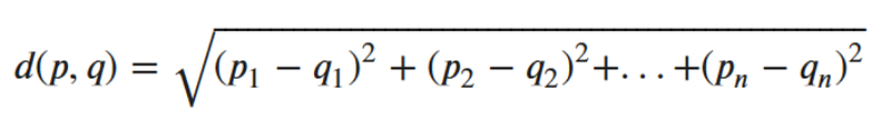
Luckily in Python, you don’t have to know the number of dimensions beforehand:

def euclidean_dist(v1, v2):
    v1, v2 = np.array(v1), np.array(v2)
    distance = 0
    for i in range(len(v1) -1):
        distance += (v1[i] - v2[i]) **2

    return np.sqrt(distance)

In our predict() method, we implement the algorithm’s ability to classify. You may notice there are a few more steps in this method than in our previous ones. Inside the predict method we:

1. Utilize our euclidean_dist() method to calculate the distance between the test_instance and each row of the train_set

2. Sort the distances from lowest to highest by value

3. Keep the k smallest distance

4. Get the values of a class variable for train_set rows with k smallest distance — these are the nearest neighbors’ values to our mystery flower and have the most similar features.

5. Determine the majority class among train_set rows with k smallest — this is our classification prediction.

6. Return prediction of sorted classes — hands the value back to the caller.

def predict(self, train_set, test_instance):
    distances = []
    for i in range(len(train_set)):
        dist = self.euclidean_dist(train_set[i][:-1], test_instance)
        distances.append((train_set[i], dist))
        distances.sort(key=lambda x: x[1])
    
    neighbors = []
    for i in range(self.k):
        neighbors.append(distances[i][0])

    classes = {}
    for i in range(len(neighbors)):
        response = neighbors[i][-1]
        if response in classes:
            classes[response] +=1
        else:
            classes[response] =1

    sorted_classes = sorted(classes.items(), key=lambda x: x[1], reverse=True)
    return sorted_classes[0][0]

Let’s test our algorithm to see how well it performed on the training data.

def evaluate(y_true, y_pred):
    correct = 0
    for actual, pred in zip(y_true, y_pred):
        if actual == pred:
            correct +=1
            return correct / len(y_true)

# Driver Code for Evaluation
train_set, test_set = train_test_split(dataset)print(len(train_set), len(test_set))

knn = KNearestNeighbors(k=3)
preds = []

for row in test_set:
    preds_only = row[:-1]
    prediction = knn.predict(train_set, preds_only)
    preds.append(prediction)

actual = np.array(test_set)[:, -1]
knn.evaluate(actual, preds)

print(knn.evaluate)

k_evaluations = []

for k in range(1, 26, 2):
    knn = KNearestNeighbors(k=k)
    preds = []

    for row in test_set:
        preds_only = row[:-1]
        prediction = knn.predict(train_set, preds_only)
        preds.append(prediction)

curr_accuracy = knn.evaluate(actual, preds)
k_evaluations.append((k, curr_accuracy))

print(k_evaluations)
# Note: 0.967 is a good score for this dataset

The From Scratch model performs well with an accuracy score of 0.9459 and a cross-validation score of 0.9729. This means the model is predicting the correct class for the flower about 96% of the time. At this point, we would typically iterate on the model, hyper-tuning parameters until we optimize efficiencies within the model to achieve optimal performance. However, today we will look at the same algorithm implemented using the SciKit-Learn library.

Test From Scratch K-NN Algorithm Against SciKit Learn K-NN Algorithm

SciKit-Learn is a free software machine learning library for the Python Programming language. It contains efficiency tools for machine learning and statistical modelings such as classification, regression, clustering, and dimensionality reduction.

To reproduce the SkiKit-Learn model, will need to import the following packages:

● from sklearn.datasets import load_iris

● from sklearn.pipeline import make_pipeline

● from sklearn.model_selection import train_test_split

● from sklearn.preprocessing import MinMaxScaler

● from sklearn.neighbors import NeighborhoodComponentsAnalysis

● from sklearn.neighbors import KNeighborsClassifier

● from sklearn.metrics import accuracy_score

● from sklearn.model_selection import cross_val_score

Note: The dataset’s loading using the SkiKit-Learn package is not displayed in this article.

The following model is operating within a K-NN Python class. It is set up just like we did in our From Scratch algorithm.

n_neighbors = 3
random_state = 42
 
# load dataset
X = dataset
y = dataframe["class"]
 
# split into train/test set
X_train, X_test, y_train, y_test = train_test_split(
        X, y, test_size=0.67, random_state=42, stratify = y
)
 
# reduce dimensions to 2 with neighborhood component analysis
nca = make_pipeline(
    MinMaxScaler(),
    NeighborhoodComponentsAnalysis(n_components=2, 
                           random_state=random_state)
    )
 
# use nearest neighbor classifier to evaluate  the methoda
knn =  KNeighborsClassifier(n_neighbors=n_neighbors)
 
# fit the method's model
nca.fit(X_train, y_train)
 
# fit nearest neighbor classifier on training set
knn.fit(nca.transform(X_train), y_train)
 
# predict the class labels for the provided data
knn.predict(nca.transform(X_train))
 
# return probability estimates for the test data
knn.predict_proba(nca.transform(X_test))
 
# calculate the nearest neighbor accuracy on the test set
knn_accuracy_sklearn = knn.score(nca.transform(X_test), y_test)
 
# calculate the nearest neighbor cross validation score on test set
scores = cross_val_score(knn, X_train, y_train, cv=5)
 
print(f'Accuracy Score: {knn_accuracy_sklearn}')
print(f'Cross-validation Score: {np.mean(scores)}')
# Note:  0.967 is a good score for this dataset

The SciKit-Learn model is performing well with an accuracy score of 0.9702 and a cross-validation score of 0.98. This means the model is predicting the correct class for the flower about 97.5% of the time.

K-NN Machine Learning Use Cases

…And Limitations

As you observed in the demonstration above, K-NN is a reasonably straight-forward algorithm that makes your model more intelligent. This is the magic of machine learning! You may be wondering, “What are some real-world applications for K-NN other than taxonomy?”

Recommender Systems

Think about Netflix, Spotify, or The New York Times App. What do they all have in common? They recommend movies, songs, or news articles to you. How do they figure out which ones to recommend to you? This is a business problem with a K-NN component to the solution. They collect information on your preferences, group you with people with similar tastes, make recommendations to you based on the closest users. K-NN may be part of the overall algorithm and used only as a jumping-off point, and the logic is at the core of the solution process.

OCR

OCR stands for optical character recognition. It allows your computer to read a text page as an image and then translate it to text. While OCR is a complex task, it’s built on simple logic. Part of the logic includes measuring and extracting features like lines, points, and curves from two characters, like a 1 and 3. You then compare each character’s features to know the characters and each other to classify the characters. This, too, involves the K-NN logic.

Limitations

Predicting the weather or the stock market are highly challenging because so many variables are involved. There is no linear correlation in either sphere that would allow us to use past data to predict future performance. Any such industry or sphere heavily influenced by randomness or ambiguity is not a candidate for K-NN logic.

K-NN Challenge

Complete this exercise on your own:

● using cosine distance instead of Euclidean distance

● standardize the data (for practice for real-world data sets where you will need to do this more often than not)

● post link(s) to your project(s) in the comments that tell me about your experience, what you find easy/challenging, what you learn, your results, etc.

I hope this gives you a foundation or fills in a few gaps regarding K-Nearest Neighbors and Machine Learning.

My Papaw always told me I’d be judged by the company I kept. I wonder what he would think about K-NN in Machine Learning!

Resources:

Bhargava, A. Y. (2016). Grokking Algorithms: An Illustrated Guide for Programmers and Other Curious People. Manning Publications.

Guttag, J. V. (2016). Introduction to Computation and Programming Using Python with Application to Understanding Data (2nd ed.). Massachusetts Institute of Technology.

Skiena, S. S. (2020). The Algorithm Design Manual (3rd ed.). Springer Nature.