It’s NeRF From Nothing: Build A Complete NeRF with PyTorch

A tutorial for how to build your own NeRF model in PyTorch, with step-by-step explanations of each component

[Note: this article includes a Google Colab notebook. Feel free to use it if you wish to follow along.]

Introduction

NeRF Explosion

The Neural Radiance Field, or NeRF, is a fairly new paradigm in the world of deep learning and computer vision. Introduced in the ECCV 2020 paper “NeRF: Representing Scenes as Neural Radiance Fields for View Synthesis” (which received an honorable mention for Best Paper), the technique has since exploded in popularity and has received nearly 800 citations thus far[1]. The method marks a dramatic change from the conventional ways by which machine learning handles 3D data. The visuals certainly have that “wow” factor as well, which you can see on the project page and in their original video (below).

In this tutorial, we will walk through the essential components of a NeRF and how to put them all together to train our own NeRF model. Before we get started, however, let’s first take a look at what a NeRF really is and what makes it such a breakthrough.

What is a NeRF?

In short, a NeRF is a generative model of sorts, conditioned on a collection of images and accurate poses (e.g. position and rotation), that allows you to generate new views of a 3D scene shared by the images, a process often referred to as “novel view synthesis.” Not only that, it explicitly defines the 3D shape and appearance of the scene as a continuous function, with which you can do things like generate a 3D mesh via marching cubes. One thing you may find surprising about NeRFs: although they learn directly from image data, they use neither convolutional nor transformer layers (at least not the original). An understated benefit of NeRFs is compression; at 5–10MB, the weights of a NeRF model may be smaller than the collection of images used to train them.

The proper way to represent 3D data for machine learning applications has been a subject of debate for many years. Many techniques have emerged, ranging from 3D voxels to point clouds to signed distance functions (for more details on some common 3D representations, see my MeshCNN article). Their big common drawback is an initial assumption: most representations require a 3D model, requiring you to either produce 3D data using tools like photogrammetry (which is very time- and data-hungry) and LiDAR (which is often expensive and tricky to use) or to pay an artist to make a 3D model for you. In addition, many types of objects, such as highly reflective objects, “mesh-like” objects such as bushes and chain-link fences, or transparent objects are impractical to scan at scale. 3D reconstruction methods often have reconstruction errors as well which can cause stair-stepping effects or drift that impact the accuracy of the model.

NeRFs by contrast rely on an old yet elegant concept called light fields, or radiance fields. A light field is a function that describes how light transport occurs throughout a 3D volume. It describes the direction of light rays moving through every x=(x, y, z) coordinate in space and in every direction d, described either as θ and ϕ angles or a unit vector. Collectively they form a 5D feature space that describes light transport in a 3D scene. The NeRF, inspired by this representation, attempts to approximate a function that maps from this space into a 4D space consisting of color c=(R,G,B) and a density σ, which you can think of as the likelihood that the light ray at this 5D coordinate space is terminated (e.g. by occlusion). The standard NeRF is thus a function of the form F : (x,d) -> (c,σ).

The original NeRF paper parameterizes this function with a multilayer perceptron trained directly on a set of images with known poses (which can be obtained via any structure-from-motion application such as COLMAP, Agisoft Metashape, Reality Capture, or Meshroom). This is one method in a class of techniques called generalized scene reconstruction, which aim to describe a 3D scene directly from an ensemble of images. This approach gives us some very nice properties:

• Learns from data directly
• Continuous representation of the scene allows for very thin and complex structures such as leaves of a tree or meshes
• Implicitly accounts for physical properties like specularity and roughness
• Implicitly represents lighting in a scene

A litany of papers have since sought to expand the functionality of the original with features such as few-shot and one-shot learning[2, 3], support for dynamic scenes[4, 5], generalizing the light field into feature fields[6], learning from uncalibrated image collections from the web[7], combining with LiDAR data[8], large-scale scene representation[9], learning without a neural network[10], and many more. For some great overviews of NeRF research, see this great overview from 2020 and another overview from 2021 both by Frank Dellaert.

NeRF Architecture

With this function alone, it is still not readily apparent how you can generate novel images. Overall, given a trained NeRF model and a camera with known pose and image dimensions, we construct a scene by the following process:

1. For each pixel, march camera rays through scene to gather a set of samples at (x, d) locations.
2. Use (x, d) points and viewing directions at each sample as input to produce output (c,σ) values (essentially rgbσ).
3. Construct an image using classical volume rendering techniques.

The radiance field function is only one of several components that, once combined, allow you to create the visuals seen in the video you saw earlier. There are several more components, each of which I will visit in the tutorial. Overall we will cover the following components:

• Positional encoding
• The radiance field function approximator (in this case, an MLP)
• Differentiable volume renderer
• Stratified sampling
• Hierarchical volume sampling

My intent for this article is maximum clarity, so I have extracted the key elements of each component into the most concise code possible. I have used the original implementation by GitHub user bmild and PyTorch implementations from GitHub users yenchenlin and krrish94 as references.

Tutorial

Positional Encoder

Much like the insanely popular transformer model introduced in 2017[11], the NeRF also benefits from a positional encoder as its input, albeit for a different reason. In short, it maps its continuous input to a higher-dimensional space using high-frequency functions to aid the model in learning high frequency variations in the data, which leads to sharper models. This approach circumvents the bias that neural networks have towards lower frequency functions, allowing NeRF to represent sharper details. The authors refer to a paper at ICML 2019 for further reading on this phenomenon[12].

If you are familiar with positional encoders, the NeRF implementation is fairly standard. It has the same alternating sine and cosine expressions that are a hallmark of the original.

Radiance Field Function

In the original paper, the radiance field function was represented by the NeRF model, a fairly typical multilayer perceptron that takes encoded 3D points and view directions as inputs and returns RGBA values as outputs. While this paper uses a neural network, any function approximator can be used here. For instance, a follow-up paper by Yu et al. called Plenoxels uses a basis of spherical harmonics instead for orders of magnitude faster training while achieving competitive results[10].

The NeRF model is 8 layers deep with feature dimension of 256 for most layers. A residual connection is placed at layer 4. After these layers, the RGB and σ values are produced. The RGB values are further processed with a linear layer, then concatenated with the view directions, then passed through yet another linear layer before finally being recombined with σ at the output.

Differentiable Volume Renderer

The RGBA output points are in 3D space, so to composite them into an image we need to apply the volume integration described in Equations 1–3 in Section 4 of the paper. Essentially, we take the weighted sum of all samples along the ray of each pixel to get the estimated color value at that pixel. Each RGB sample is weighted by its alpha value. Higher alpha values indicate higher likelihood that the sampled area is opaque, therefore points further along the ray are likelier to be occluded. The cumulative product ensures that those further points are dampened.

Stratified Sampling

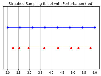
In this model, the RGB value that the camera ultimately picks up is the accumulation of light samples along the ray passing through that pixel. The classical volume rendering approach is to accumulate and then integrate points along this ray, estimating at each point the probability that the ray travels without hitting any particle. Each pixel therefore requires a sampling of points along the ray passing through it. To best approximate the integral, their stratified sampling approach is to divide the space evenly into N bins and draw a sample uniformly from each. Rather than simply drawing samples at regular spacing, the stratified sampling approach allows the model to sample a continuous space, therefore conditioning the network to learn over a continuous space.

Hierarchical Volume Sampling

Earlier when I said that the radiance field is represented by a multilayer perceptron, I may have lied a little. In fact, it’s represented by two multilayer perceptrons! One operates at a coarse level, encoding broad structural properties of the scene. The other refines the details at a fine level, thus enabling thin and complex structures like meshes and branches to be realized. In addition, the samples they receive are different, the coarse model processing broad, mostly regularly spaced samples throughout the ray, and the fine model honing in on areas with strong priors for salient information.

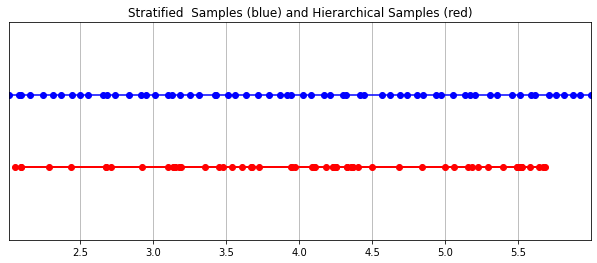
This “honing in” process is accomplished by their hierarchical volume sampling procedure. The 3D space is in fact very sparse with occlusions and so most points don’t contribute much to the rendered image. It is therefore more beneficial to oversample regions with a high likelihood of contributing to the integral. They apply learned, normalized weights to the first set of samples to create a PDF across the ray. They then apply inverse transform sampling to this PDF to gather a second set of samples. This set is combined with the first set and fed to the fine network to produce the final output.

Training

The standard approach to training NeRF from the paper is mostly what you would expect, with a few key differences. The recommended architecture of 8 layers per network and 256 dimensions per layer can consume a lot of memory during training. Their approach to alleviate this is to chunk the forward pass into smaller pieces and then accumulate the gradients across these chunks. Note the distinction from minibatching; the gradient is accumulated across a single minibatch of sampled rays, which may have been gathered in chunks. If you do not have an NVIDIA V100 GPU as was used in the paper or something with comparable performance, you will probably have to adjust your chunk sizes accordingly to avoid OOM errors. The Colab notebook uses a much smaller architecture and more modest chunking sizes.

I personally found NeRFs somewhat tricky to train due to local minima, even with many of the defaults chosen. Some techniques that helped include center cropping during early training iterations and early restarts. Feel free to try different hyperparameters and techniques to further improve training convergence.

Conclusion

Radiance fields mark a dramatic change in the way machine learning practitioners approach 3D data. The NeRF model, and more broadly differentiable rendering, are quickly bridging the gap between creation of images and creation of volumetric scenes. While the components we walked through may seem very intricately assembled, countless other methods inspired by this “vanilla” NeRF prove that the basic concept (continuous function approximator + differentiable renderer) is a strong foundation upon which to build a variety of solutions tailored to nearly limitless situations. I encourage you to give it a try for yourself. Happy rendering!

References

[1] Ben Mildenhall, Pratul P. Srinivasan, Matthew Tancik, Jonathan T. Barron, Ravi Ramamoorthi, Ren Ng — NeRF: Representing Scenes as Neural Radiance Fields for View Synthesis (2020), ECCV 2020

[2] Julian Chibane, Aayush Bansal, Verica Lazova, Gerard Pons-Moll — Stereo Radiance Fields (SRF): Learning View Synthesis for Sparse Views of Novel Scenes (2021), CVPR 2021

[3] Alex Yu, Vickie Ye, Matthew Tancik, Angjoo Kanazawa — pixelNeRF: Neural Radiance Fields from One or Few Images (2021), CVPR 2021

[4] Zhengqi Li, Simon Niklaus, Noah Snavely, Oliver Wang — Neural Scene Flow Fields for Space-Time View Synthesis of Dynamic Scenes (2021), CVPR 2021

[5] Albert Pumarola, Enric Corona, Gerard Pons-Moll, Francesc Moreno-Noguer — D-NeRF: Neural Radiance Fields for Dynamic Scenes (2021), CVPR 2021

[6] Michael Niemeyer, Andreas Geiger — GIRAFFE: Representing Scenes as Compositional Generative Neural Feature Fields (2021), CVPR 2021

[7] Zhengfei Kuang, Kyle Olszewski, Menglei Chai, Zeng Huang, Panos Achlioptas, Sergey Tulyakov — NeROIC: Neural Object Capture and Rendering from Online Image Collections, Computing Research Repository 2022

[8] Konstantinos Rematas, Andrew Liu, Pratul P. Srinivasan, Jonathan T. Barron ,Andrea Tagliasacchi, Tom Funkhouser, Vittorio Ferrari — Urban Radiance Fields (2022), CVPR 2022

[9] Matthew Tancik, Vincent Casser, Xinchen Yan, Sabeek Pradhan, Ben Mildenhall, Pratul P. Srinivasan, Jonathan T. Barron, Henrik Kretzschmar — Block-NeRF: Scalable Large Scene Neural View Synthesis (2022), arXiv 2022

[10] Alex Yu, Sara Fridovich-Keil, Matthew Tancik, Qinhong Chen, Benjamin Recht, Angjoo Kanazawa — Plenoxels: Radiance Fields without Neural Networks (2022), CVPR 2022 (Oral)

[11] Ashish Vaswani, Noam Shazeer, Niki Parmar, Jakob Uszkoreit, Llion Jones, Aidan N. Gomez, Lukasz Kaiser, Illia Polosukhin — Attention Is All You Need (2017), NeurIPS 2017

[12] Nasim Rahaman, Aristide Baratin, Devansh Arpit, Felix Draxler, Min Lin, Fred A. Hamprecht, Yoshua Bengio, Aaron Courville — On the Spectral Bias of Neural Networks (2019), Proceedings of the 36th International Conference on Machine Learning (PMLR) 2019